Cosine similarity

Embedding words as numeric vectors enables estimates of semantic similarity

In my coursework on large language models (LLMs)—where I’m a beginner—I encountered an unfamiliar term, cosine similarity. It’s a useful metric and a good excuse to quickly illustrate how language models bridge the gap from words to numbers. Here is the code; as usual, I write in R rather than python. This simple exercise reduces to four steps:

1. Define two word vectors (arbitrarily defined by me)

2. Load pre-trained word vectors from GloVe’s public dataset (or here at github)

3. Lookup my words in GloVe’s database and retrieve each word’s embedding: a 50-dimensional numeric vector the represents the word.

4. Compute the pairwise cosine similarities. This is similar to a correlation matrix where instead we’ve estimated semantic similarity but in the same unitless scale, from -1.0 to +1.0.

For the first step, my two vectors are self-selected finance and economics terms (some terms like ETF, hedge funds, and IPO are not to be found in this particular dictionary):

vector3_words <- c("stocks", "bonds", "options", "commodities", "rates", "derivatives", "forex", "dividends", "profits", "bitcoin") 

vector4_words <- c("economy", "growth", "recession", "inflation", "employment", "trade", "policy", "taxation", "savings", "investment", "credit", "bubble", "crisis")

For step 2, see code (the only issue is file size). Step 3 is just a lookup (of words in my vectors) into the GloVe dataset. This yields a matrix where each row is a word (e.g., “stocks”) with 50 features (or columns). That’s the essential mutation that underlies the exercise. Each word is represented by 50 dimensions (V1, V2, … , V50) that are themselves abstract:

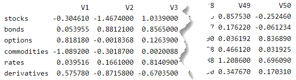
And here is a heatmap of the pairwise cosine similarities:

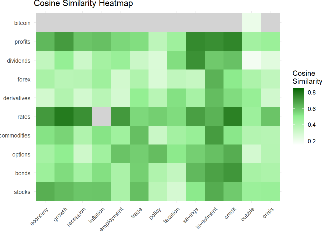
So that’s a trivial illustration of an underlying LLM dynamic:

Words are represented (via embedding) as long (aka, high-dimensional) numeric vectors which enables similarity measurement; e.g., “profits” is more similar to “investment” (0.7358) than to “policy” (0.367) because the profit/investment angle is ~42 degrees while the profits/policy angle is ~68 degrees.

The matrix math for cosine similarity is pretty basic (see code) but it’s a reminder: if you want to learn anything about LLMs, you’ll encounter linear algebra. In fact, I can’t avoid python or linear algebra (so I’m learning some python despite a decade invested in learning R).

Illustrated with 2D vectors

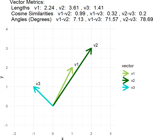
For a glorious video on cosine similarity, see Josh Starmer. Below is my ggplot illustration of the concept with super-short vectors (see the “appendix” to my same code).

# Define three vectors 
v1 <- c(1, 2) 
v2 <- c(2, 3) 
v3 <- c(-1, 1)

The point is, visually you likely consider all three vectors to be dissimilar; i.e., relative to v1, v2 is longer and v3 is almost orthogonal. But cosine similarity does not care about the vector’s magnitude; it only cares about the angle between the vectors. The angle between v1 and v2 is only about 7 degrees, so they are highly similar and their cosine similarity is 0.99.