
Decision tree introduction (with code) to predict dividend or loan default, Part 1
At each node, the training data branches (splits) into two subsets, divided by the feature with most information-to-gain about the target variable. High interpretability at the risk of overfitting.

Contents
Predict Dividend (yes/no) with four features. The key is to understand that a node splits a group by the feature with the most information-to-gain about the target
Predict loan default with 16 features. Train the model, then test the model: evaluate with a confusion matrix. Add penalties to avoid expensive errors.
I've been writing practice questions (PQs) for the FRM's new machine learning readings. Next week's topic is decision trees and the syllabus wants candidates to be able to "show how a decision tree is constructed and interpreted." Many data scientists seems to agree that trees are interpretable1 (pro) but tend to overfit (con).
You can view my code + exhibits at this Quarto document on my finedtech.io site.
1. Predict Dividend (yes/no) with four features
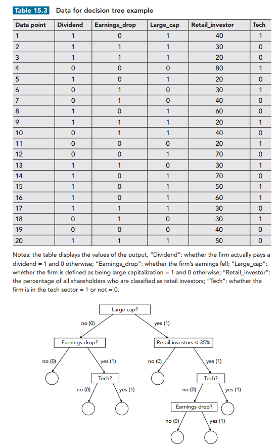
Below is a snapshot of the dataset and an illustration of its first split. The setup2 is a small sample (n = 20) of public company observations (left panel). The target variable is Dividend ("Div" in red): firms either paid a dividend (Div = 1) or did not pay a Dividend (Div = 0). This is why decision trees are called supervised learning: we’re able to label the dependent variable in the training set. Each company has four features. Three are simple binaries: Earnings (1 = dropped in last period), LargeCap (1 = yes), and Tech (1 = yes). Retail—the fourth feature—is the percentage of retail investors.
Before we consider any features, we can see that 45% of the firms (9/20) paid a dividend. That’s pretty close to a coin flip. Information purity is measured with the Gini “impurity” coefficient. The base Gini of the entire (all 20) training set is the Gini before we split on any features. Here, the base Gini is given by 1 - (0.450^2 + 0.550^2) = 0.4950. Since these are binaries, 1 - p^2 - (1-p)^2 = 2*p*(1-p) so we can also get the base Gini with 2*(9/20)*(11/20) = 0.4950.
The decision tree is just a root node (that contains all 20) that splits into two nodes (each of which contains a subset according the first feature). Then each of those nodes might split again, and so on, until we reach a final node called a leaf. To split on a feature is just to break the node into two branches. How do we pick the feature at each node, including the root? We split on the feature with the most information-to-gain about the target variable; i.e., that offers the greatest reduction in Gini impurity3.
Below I show the information gain achieved by splitting first on the LargeCap feature, which earns that first split by its largest Gini reduction (compared to the other three features). The left panel below shows the original, unsorted set of 20 firms and its base Gini of 0.4950. The right panel sorts on LargeCap where we need a Gini coefficient for each branch (LargeCap = 1 is the upper 13 with a Gini of 0.4260, and LargeCap = 0 is the lower 7 with a Gini of 0.0000).
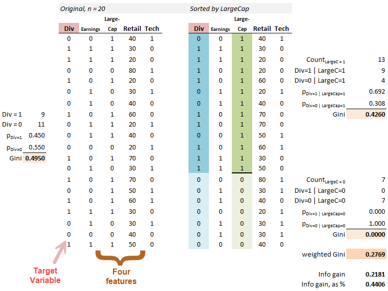
When the root splits on LargeCap, we gain some information in the branch to the 13 LargeCap companies, where Div=1|LargeCap=1 = 9. This branch gets us from 9/20 to 9/13, but notice the Gini only decreases to 0.4260. However, among the seven companies who are not LargeCap, none paid a dividend. That’s a pure node! It’s really helpful to split on this feature. Because it goes to a pure node, this branch (i.e., to the seven who are not LargeCap) earns a Gini of zero. The weighted Gini of this root split on LargeCap is therefore 0.2769 for a gain of 0.4950 - 0.2769 = 0.2181 or 0.2181/0.4950 = 44.06%.4
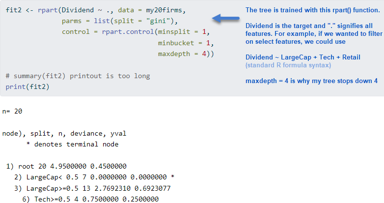
That's the essence of a decision tree: at each node, it says "based on the group in this node, let's split now on the feature that gains us the most information, if it's worth the additional complexity". Based on the parameters I gave to the rpart() function, the following tree is generated.
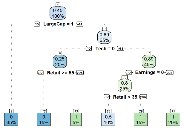
Each node has a node number (nn); some numbers are skipped because the algo has pruned the tree. At the top (nn = 1), we see that 0.45 or 45% of the total training set paid a dividend (= 9/20 paid a dividend). Because it won the Gini reduction contest at this node, LargeCap splits the root. Among those who are not LargeCap (LargeCap = 0), we follow to the left of the root and go directly to the leaf at the bottom. Because all 7 of those firms (which is 7/20 = 35%) did not pay a dividend, the tree predicts that any firm which is NOT a LargeCap will NOT pay a dividend (the 0 is the prediction for the target variable). If the firm is a LargeCap, we follow to the right of the root and encounter the next node. Before we split again, we observe the 65% here tells us that 13/20 firms are LargeCap. I think of this 65% as the size of the node (I wonder if it’s possible to size the node thusly?!). So the 100% (=20) splits 35% to the left’s leaf and 65% to this right’s node. Among these 13 that occupy this node before it splits, 9/13 = 0.6923 or 0.69 paid a dividend; that is, P(Div =1 | LargeCap = 1) = 9/13.
The Gini reduction contest says this node (this group of 13 LargeCaps) should split on the Technology feature. This 65% LargeCaps node (n = 13 of 20 total) splits into two groups: 20% (n = 4) to the left (Tech = 1) and 45% (n = 9) go to the right (Tech = 0). Among the four firms to the left, the 0.25 indicates that only 1 of the 4 paid a dividend (that’s firm on the 11th row in the right panel). And so on.
The key to a decision tree is that each node splits a subset into two (binary branches) according to the feature that offers the most information-to-gain about the target. Each leaf at the bottom is results of a series of if-then statements which can be applied to each new test or out-of-sample observation to make a prediction.
Consider the light-blue bottom leaf, nn = 28. The 10% indicates that 10%*20 = 2 firms occupy this node, and the 0.5 indicates that one of the 2 (1/2 = 0.5) paid a dividend, so the other did not. Imagine a firm in the testing set happens to be (reading from top to bottom) a LargeCap, non-Tech, Earnings (=1) dropper, with less than 35% retail ownership. Given these features, we can traverse the tree and arrive at leaf 28. This leaf predicts a 50% probability that the firm will pay a dividend. The other five leaves predict either pay (1) or not pay (0)! Why? Because those are pure nodes. Hence you can imagine the overfitting drawback potential, yes? The tree might have an ability to proliferate to mostly pure nodes but such an overgrown tree will invariably overfit the training sample.
In my code, you might notice that this is actually a regression tree. To be honest, I didn't realize until after I ran printcp(). My subsequent command …
my20firms$Dividend <- as_factor(my20firms$Dividend)
… converts the numerical (target) Dividend variable to a categorical factor. After this edit to the target, the re-trained tree becomes a classification tree, and it's also a notch simpler.
2. Predicting loan default with 16 features
My next example goes further by using the same dataset used in Machine Learning with R by Brett Lantz (4th Edition). I am almost finished reading this brilliant book; I’ll review it shortly, as it’s probably my favorite introduction to machine learning. These are German loans and the target variable is default (a binary yes/no; I colored yes in pink and repayment in green to make is easier to read). This dataset has 16 features. I didn’t have to train on all of them. But the “.” in “default ~ .” signifies that we want to train all features on the target, per the function that contains other parameters (“parms”) and controls:
tree_credit_train <- rpart(default ~ ., data = credit_train, parms = list(split = "gini"), control = rpart.control(minsplit = 1, minbucket = 1, maxdepth = 4))
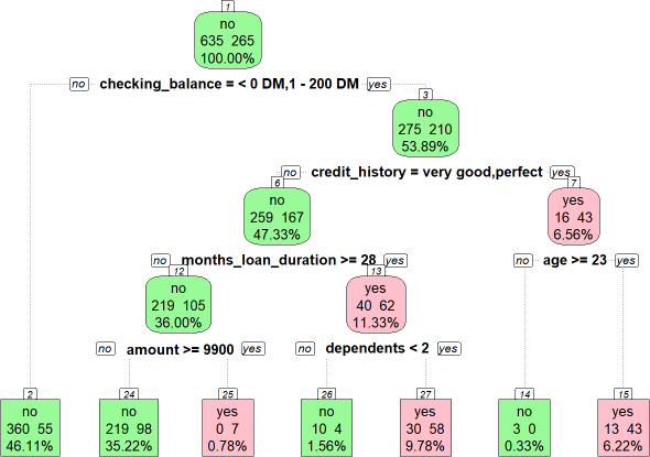
The resulting tree has an odd outcome: node (nn) 3 branches to the right for credit_history = (“very good” | “perfect”) where the prediction is default for those who are 23 years or older. But counterintuitively the lower credit (history) quality categories are more likely to repay. Such is this data5.
This time we held-out 10% for testing. With a single command, we can retrieve a vector of predictions—e.g., tree_credit_pred = {no, no, no, yes …}—with the predict() function:
tree_credit_pred <- predict(tree_credit_train, credit_test, type = "class")
Confusion matrix
The confusion matrix reveals the test results. The upper panel below shows an unimpressive accuracy of 65% (= 58 + 7). The false negative (FN) rate is fully 28/35 = 80%. Yikes. The false positive (FP) rate is 7/65 = 10.8%. Let’s assume that false negatives are the more costly error we seek to avoid. It’s easy to do this in rpart(): we define a loss matrix (zero in the diagonal where the predictions are correct) and activate it in the params list with “loss = penalty matrix”. My penalty matrix arbitrarily assigns a relative cost of 3:1. The lower panel shows the test with the revised model6:
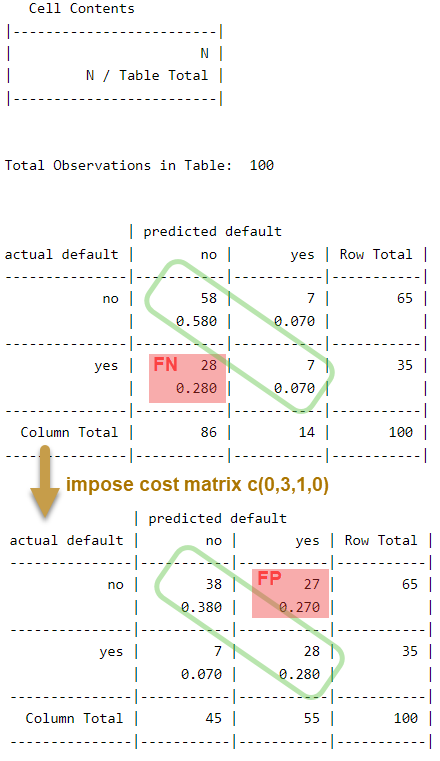
Against the same 10% test set, the new tree model reduces false negatives (FN) to 20.0%. But false positives increase to 27/65 = 41.5%.
There’s a lot more to explore but I hope this was an interesting introduction!
The interpretability of a decision tree is a huge advantage. Like a binomial tree, we can intuitively follow branches at each node. Further, unlike many ML techniques, we don’t need to scale or transform the features. Given a tree and a new test observation, we can apply the tree quickly and intuitively. Many cite an ability to easily visualize the tree. For myself, I find these advantages a bit overstated. For me, the split logic/metrics and tree parameters required quite some effort. Invariably, you can’t use the tree you get out-of-the-box, so there are tricky controls to learn and algorithmic nuances; e.g., different packages produce different trees. Even the visualization is non-trivial: I could not find a versatile ggplot2 extension.
GARP’s setup and their implied tree is shown here (Source: Table 15.3, 2023 FRM Exam Part 1, Chapter 15, Machine Learning and Predictions). I made five changes (shown in my code chunk) just to get a tree that was more interesting for the PQ:
my20firms <- garp_data
my20firms$Dividend[1] <- 0
my20firms$Dividend[9] <- 0
my20firms$Dividend[12] <- 1
my20firms$Dividend[13] <- 0
my20firms$Dividend[15] <- 0
An alternative to Gini impurity measure is information entropy. It often makes little difference which measure is used (and it made no difference in either of my examples); other tree parameters were more consequential. I followed GARP’s example and used Gini. In my Dividend example, if we were to instead use entropy, the base entropy measure is given by -[log(9/20, 2)*(9/20) + log(11/20)*(11/20)] = 0.9928. Entropy’s scale is 0 to 1, where 0 is certainty and 1.0 is peak uncertainty.
In my code, I used the rpart() function to train the tree. After the printcp(fit2) command, you'll notice first line includes the value 0.440559 which matches my 0.4406 above.
Brett Lantz got the same result (but I did use his seed value!). As shown in the code, I did re-level the factors, but that didn’t change the result. I could override this by (i) excluding the feature, (ii) pre-split on this feature, or (iii) recode/transform the feature [e.g., reduce five categories to two or three]. Brett says this about the anomaly, “Sometimes a tree results in decisions that make little logical sense. For example, why would an applicant whose credit history is perfect or very good be likely to default, while those whose checking balance is unknown are not likely to default? Contradictory rules like this occur sometimes. They might reflect a real pattern in the data, or they may be a statistical anomaly. In either case, it is important to investigate such strange decisions to see whether the tree’s logic makes sense for business use.” — Chapter 5, Brett Lantz, Machine Learning with R, Fourth Edition, 2023.
This second confusion matrix is predicting on the exact same held-out testing set (n = 100 or 10% for both tests) but the second decision tree is different because it trained with an additional consideration: information improvement via the Gini coefficient is considered along with the relative cost of making each error.