
k-fold cross-validation
Rather than validate once, k-fold CV validates once for each fold in an efficient use of a small sample. Its job is model evaluation and/or hyperparameter tuning, not parameter selection.

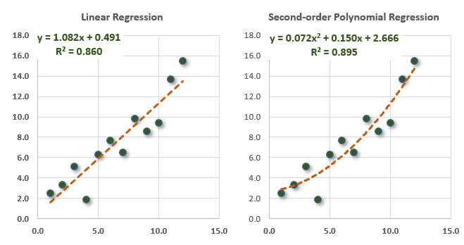
The scatterplots below are identical, but two different lines fit the data. On the left, an ordinary least squares (OLS) linear regression; on the right, a second-order polynomial regression. Here's a question: If the goal is prediction, which line is better?
In this post, I'll explain how k-fold cross validation (aka, k-fold CV) answers the question. First, I'll illustrate with an example inspired by GARP's EOC practice question. Second, I'll highlight their mistake as a means to clarify the function of a k-fold CV by elaborating on the example.
The validation set evaluates the model or tunes hyperparameters
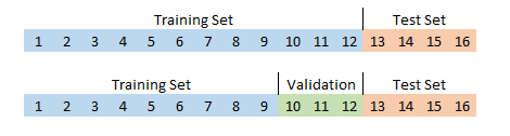
A traditional exercise splits the dataset into two parts: a training set (likely 70% to 90% of the observations) and a test set (the remaining 10% to 30%). A big, known problem in machine learning is overfitting. A popular remedy is validation. If we want to validate before testing, we can split the data into three sets: training, validation, and testing. Typical is 80%/10%/10% or 70%/15%/15%. Most of us can intuit the concept of training for the unseen test set that is said to be truly "held out", but what's the idea behind splitting into a third (validation) set?
Training set: the largest subset of the data that is used to generate the model's parameters. Put simply, a model learns on the training set.
Validation set: a smaller subset used to evaluate the model and/or tune the model's hyperparameters when we want to choose between models and/or the model(s) have hyperparameters that can be tuned. Put simply, the model meta-learns on the validation set.
Test set: the small subset that is truly independent (“held back”) from both training and validation. Because it has no influence on the model or its hyperparameters or its parameters, the test set evaluates the model on unseen data.
I'm using a linear regression model in order to relate my example to an existing GARP example, but this model does not actually have hyperparameters1: The OLS linear regression unequivocally finds the only straight line that minimizes the sum of square residuals (RSS). There is no meta-learning, there is only "learning" the line's intercept and its slope coefficient(s) from the dataset. These coefficients, often denoted β(0), β(1), … β(n), are the model's parameters2.
Hyperparameters (a brief aside)
Unlike the OLS linear regression, many machine learning models do have hyperparameters in addition to parameters. Consider the k-nearest neighbor (KNN) algorithm which is supervised learning because each observation is labeled. For example, a scatterplot of (X =) hours studied versus (Y =) number of mock exams taken by exam candidates might label each observation as {Pass | Fail}. The KNN algo classifies a new observation based on a vote among the K "nearest" students who share a similar profile3. If K = 10, then the 10 nearest student are polled; if most of those 10 neighbors passed the exam, the observation is classified (predicted to be) a Pass.
But the KNN model does not give us K. We can select any K = X neighbors. Selecting K is artful and occurs before training4. As such, this K is a hyperparameter. Hyperparameters are selected before the training and consequently, unlike the parameters, are not learned from the data. So just keep in mind that my example does not show you hyperparameter evaluation. That's the other important reason to validate. Rather, we are here use validation only to compare two different models.
k-fold cross validation helps cope with a small sample
My practice question5 was inspired by GARP's practice question on k-fold CV (GARP P1.T2.9.12). I wanted a small sample, so my arbitrary assumption is that our full dataset only contains 16 observations. This is a dilemma of too little data!6
For the test set, I've assumed we hold back four (fully 25%) in all scenarios. If this were merely a training/test split, the training set would contain the other 12 observations. If we wanted a train/validate/test split, then maybe we'd try to validate on three and train on nine:
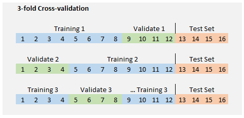
But isn't that cramped? It does not feel like we have enough data for a meaningful train/validate/test split. What we can do is collapse the training and validation sets into one set of 12 and divide this group into a desired number of "folds." If we desire three folds (i.e., on the way to a 3-fold cross-validation), then each fold holds 12 ÷ 3 = 4 observations. We can then train k = 3 times where each fold is the validation set once and only once. In the first run, observations {9, 10, 11, 12} are the validation set while {1, 2, …, 7, 8} are the training set.
Let's do that (3-fold CV) with an example
Below is similar to the exhibit I served in my practice question. The first three columns are the data. Three versions of the linear regression model (i.e., M1, M2 and M3: one for each fold) generate their respective intercept, slope and R^2. The first fold is captured under the M1 column ("version M1") of the linear regression model. This M1 version is a univariate regression trained on the first eight observations (light green) and validated on the last four (light blue). This test produces a mean squared error (MSE) of 2.02. Model version M2 regresses on observations {5, …, 12} and version M3 regresses on observations {1, 2, 3, 4, 9, 10, 11, 12} because it holds out {5, 6, 7, 8} for the validation.
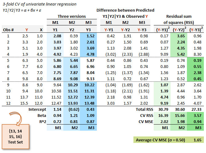
GARP's solution selects the version with the smallest RSS (in my example, that would be model M3) on a theory that we'd use the coefficients of the winning model. But this is an incorrect application of k-fold CV: if we really do prefer to use the univariate linear regression model, why would we settle for coefficients trained on half of the data? (In addition to the 4 held out for validation, recall we held out 4 as the genuine testing set).
The correct procedure here is to evaluate this model by retrieving the average MSE; in this case, the average MSE is 1.65 (with standard deviation of 0.50). That's their key procedural mistake. In GARP's solution the M3 version of the model wins, so they would use these coefficients (i.e., intercept of 0.430 and slope of 1.088). But there is only one model here (univariate linear regression) that is run on three different subsets (one for each fold). That's why I labeled them "versions" rather than "models": three versions of one model. Different data subsets generate different coefficients, obviously. But these winning coefficients (0.430 and 1.088) are based on only 8/16 = 50% of full dataset and 8/12 = 66.67% of the non-test dataset. The M1, M2 and M3 results each contribute toward evaluation of the model. If this model wins, then we (after "discarding" these results) want to fit it to the full set of 12 non-test observations.
The k-fold CV performs k validations for each version of the model and a given set of hyperparameters; then we switch the model and/or hyperparameters and do it again. We do not perform k-fold cross-validation in order to validate parameters (because parameters want to be training on the full non-test dataset). We do perform k-fold cross-validation in order to evaluate hyperparameters and/or evaluate models. If the only thing we have here is a univariate regression model, we don't need k-fold cross-validation.
Let's compare the to a polynomial regression on the same data
So let's go further and imagine that we want to compare the linear regression to a second-order polynomial regression. Notice this is a comparison between different models (i.e., linear versus polynomial regression). Using the same dataset, I show those coefficients below. The only difference is that (below) an additional coefficient is generated for the extra X^2 term. The right-half of the exhibit is structurally identical.
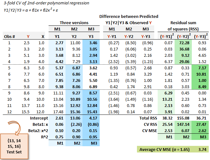
You can see that the average MSE of this model is 3.74; that's more than twice the linear model's average MSE of 1.65. In this 3-fold CV, the linear regression beats the polynomial regression. Notice this finding contradicts the fact that the polynomial regression wins on the overall set of 12 with a higher R^2 (and therefore lower RSS, and therefore lower MSE given the sample size is the same).
This is how to use k-fold CV: it tells us to prefer the linear regression model. Or at least we can say: motivated to help us avoid overfitting, it gives the means and a metric by which to decide. By training K versions of the model--with each fold serving as the validation set exactly once--we employ a defense against the overfitting problem. I would summarize the k-fold CV thusly:
Rather the validate on a single held-out set (i.e., held-out for validation prior to the testing hold-out), we get to validate k times in an organized way (once for each fold).
Am I now able to reveal to you whether this was the correct decision? No, I cannot! I did not bother to generate the final four genuine test observations: they could be anything, they are truly out-of-sample. I hope that was helpful!
P.S. After I published this post, I received this email response: “Very good analysis, but what exactly is the conclusion? Basic common sense dictates that if you represent the relationship of a scatter plot with a quadratic, then there are more chances of over fitting as compared to representing a relationship with a line (say OLS method). You can choose a model based on higher R^2 or lower MSE based on your judgement, but I think here you are suggesting a rule.”
My reply: “No, I am not suggesting a rule. I am merely using the two models to illustrate the k-fold cross-validation, a techniques that I only learned myself in order to write a practice question (and inspired by GARP’s misunderstanding of their own assignment, as noted in the post!). I like that the k-fold CV decisively favors the straight line despite the polynomial’s higher R^2. I agree with you about using judgment, of course. The only purpose here is to illustrate k-fold CV. I don’t suggest it should decide either. Thank you.”
Although I suppose it is technically untrue, I tend to think of the regression intercept as a hyperparameter in those cases where we have an interpretation for the zero y-intercept. For example, in the CAPM (or ICAPM or APT, for that matter), we often have a good reason to insist that E(alpha) = zero and constrain the y-intercept to zero. This is a prior-to-training choice.
I studied econometrics before machine learning so the term parameters often confuses me. In statistics, estimators (the mathematical recipes) generate estimates from samples, and samples vary; the estimates are trying to infer the unseen population parameters. In a univariate regression, the theory is that there exists a single population regression function (PRF) with a single slope parameter; then each sample generates a different sample regression function (SRF) such that sample estimates are random variables. In this way, when machine learning refers to a parameter, I’m often thinking “wait, that’s just a coefficient (or estimate).”
What does it mean to be “near” another students (as a neighbor in KNN)? In the two-dimensional example, that can be the length of a straight line as measured by Euclidian distance. Euclidian distance generalizes to multiple dimensions. And there are other measures of distance.
Technically, KNN is so-called lazy learner (see Brett Lantz)
Here is my practice question: “23.1.3. Charles has a small sample of only 16 monthly observations. Due to the sample size and that he is undecided on which type of model to utilize, he wants to apply the technique of k-fold cross-validation. His ultimate hold-out (testing) set will include four months such that his cross-training set (aka, training plus validation) will include only 12 observations. His first model is a simple univariate linear regression, and that analysis is displayed below. He selects k = 3 folds such that each fold in his 3-fold cross-validation includes 12/3 = 4 observations (excluding the hold-out testing set of 4 months). The three versions of the linear regression (M1, M2, and M3) are each trained on eight observations (see the green cells). This enables him to compute their respective out-of-sample sum of squared residuals (aka, CV RSS in blue cells); similarly, the mean squared error (MSE) for each model is displayed.”
« Insert first table here»
Charles observes that the third version of the univariate linear regression (i.e., M3) has the lowest CV RSS. Given this context, which of the following statements is TRUE about his 3-fold cross-validation?
a. A proper k-fold cross-validation technique computes the average MSE; specifically, (2.02 +1.98 +0.94)/3 =1.65; and compares this performance to his alternative models
b. His mistake is that, given the sample size is only 12, he should instead select k = four folds with 12/4 = three observations per fold
c. The drawback of his approach is that the bias-variance tradeoff implies that the model with the lowest residual sum of squares (RSS) is likely to have the highest mean squared error (MSE), and this subjectivity is a disadvantage of k-fold cross-validation
d. The mistake in his methodology is that each of his three models should instead train on only four observations (rather than eight) so that each can validate on the next four observations and test on the remaining four observations; i.e., 4 train + 4 validate + 4 test = 12 total observations”
You’ll notice my X-axis is just a sequence from {1, 2, …, 11, 12} which is not realistic, unless these are meant to be sequential time periods. I didn’t mean anything except it was easy for me. Only after I added the polynomial regression did I realize why the k-fold cross-validation “penalizes” the polynomial for overfitting. Notice how the polynomial’s intercepts are {2.61, 4.17 and 13.06}. The M2 version that trains on the right-side of the scatterplot (the higher eight) really “overshoots” the lower four. The linear model, on the other hand, overshoots only a little due to its lack of curvature. This was not my intention beforehand (as the PQ itself never adds a polynomial model but only alludes to GARP’s mistake), but I like the illustration.