

The link between beta and diversification, academically speaking (2nd in Series)
The link between beta and diversification, academically speaking (2nd in Series)
Within the portfolio, low marginal volatility positions confer diversification benefit. Against an index, low-beta positions pull down the average beta and are likely to have lower specific risk.

Previously I wrote an article, What is equity beta?. The point was to answer a forum member’s question (quoted in full at the link) that reduces to, What’s the link between beta and diversification? That article deep dived into beta. The goals were (i) to clarify why we can refer to beta as a scaled correlation, and (ii) to remind that beta is a regression slope with respect to some variable among several possibilities. I’ll now continue and finally answer the question! Two notes about the following:
Below considers both major types of beta: with respect to the portfolio, and with respect to an index that proxies the market
The perspectives below are insufficient for me as an investor. Why? It’s merely the math in frameworks given their assumptions. It would be useful if I trusted the covariance matrix and each stock’s beta to persist; if I depended on the mean-variance framework; if I relied on the SML and CML in practice. But I don’t. So below is an academic reply, not a realistic response. To practice diversification in a real portfolio is a hard practice.1 Still, Picasso said, “we should learn the rules like a pro, so [we] can break them like an artist.”
Beta with respect to the portfolio
My previous beta explainer assumed the classic two-asset portfolio. Here I’ll extend to three assets if only to show we can generalize to multiple assets via matrix algebra. I’m accustomed to spending a lot time tweaking assumptions in service of usable illustrations, but GPT4 gave me useful illustrative assumptions on the first try2. Wow! Those assumptions are:
Apple (AAPL) with 25% volatility
Coca-cola (KO) with 15% volatility
Exxon Mobil (XOM) with 20% volatility
Correlations: ρ(AAPL, KO)= 0.30; ρ(AAPL, XOM)= 0.40; ρ(KO, XOM)= 0.25
Under equal weights (1/3rd each), those assumptions are displayed below. The covariance matrix translates the correlations per COV(X,Y) = σ(X)*σ(Y)*ρ(X,Y); e.g., COV(APPL,XOM) = 25%*20%*0.40 = 0.0200. This equally-weighted portfolio’s volatility is sqrt(0.0225) = 15.0%3. Thank you GPT for round numbers on the first try!

Marginal volatility (aka, marginal contribution to risk, MCR)—a unitless first derivative—is the sensitivity of the portfolio volatility to a change in the asset’s weight. Each stock in the portfolio has a marginal volatility. For example, Δ(AAPL) = 0.2083 implies that adding 1.0% to the AAPL position will increase portfolio volatility +0.2083%4. Marginal volatility, Δ(i, P), is given by:
The component volatility (aka, contribution to risk, RC) translates marginal volatility into an intuitive contribution to the portfolio volatility. Marginal volatility multiplied by the position’s weight returns the position’s contribution. For example, in AAPL’s case, Δ(AAPL, P) of 0.2083 * 33.3% weight = 6.94% and the total portfolio volatility of 15.00% = AAPL’s 6.94% + KO’s 3.06% + XOM’s 5.00%.
The beta of the position (with respect to the portfolio), β(i, P), is given by the usual covariance/variance fraction (explained in the second half of the previous article). We can cancel portfolio volatility to retrieve an elegant expression: beta is marginal contribution divided by portfolio volatility; e.g., XOM’s marginal volatility of 0.1500 divided by portfolio volatility of 15.00% returns beta of 1.00:
The correlation of the position (to the portfolio that includes the position) is beta multiplied by the cross-volatility (aka, scaled by relative volatility):
And we’ve arrived at a mathematical understanding of (the first part of) an answer to the question:
Higher beta (with respect to the portfolio) is directly proportional to higher correlation. Diversification is the benefit of imperfect (lower) correlation. To add more of a high-beta stock (e.g., AAPL’s 1.3780) is to add more of a highly correlated stock (e.g., AAPL’s 0.8383) and that increases portfolio volatility. More directly, marginal volatility is the key prism and it is a function of the covariance matrix: a low-beta stock confers diversification benefit (aka, lower portfolio volatility) because it has lower pair-wise correlation with the portfolio’s other stocks.
It didn’t occur to me until I wrote these words but we can inspect the covariance matrix and retrieve the row sums (or the columns sums, equivalently). Each position thusly has a sum of its pairwise covariances (that includes its own variance). KO has the lowest row sum at 0.0113 + 0.0225 + 0.0075 = 0.0413; i.e., compared to sum(XOM) = 0.0675 and sum(AAPL) = 0.0938. This low value is a semi-usable indicator of why XOM confers diversification benefit.5
Beta with respect to the market index
Now I will switch to the more familiar beta: instead of the above β(i,P), I’ll now refer to β(i,M) which is a measure of systematic risk. It’s not grandly different: it’s still a scaled correlation but to a market index variable (itself a proxy for the market if we want to access the full theory) rather than a portfolio. There is already extensive theory, I have nothing novel to add. But I haven’t before seen the visual linkage (see below) between the capital market line (CML) and a security market line (SML) which explicates the role of specific (aka, idiosyncratic) risk in their relationship.
The construct is common in teaching. We only need six assumption to populate both CML and SML, in this case:
For Asset A, μ(A) = +10.0%, σ(A) = 10.0%.
For Asset B, μ(B) =+16.0%, σ(B) = 20.0%.
Their correlation, ρ(A,B) = 0.30, and the riskfree rate is 6.0% (to give the plots strong features).
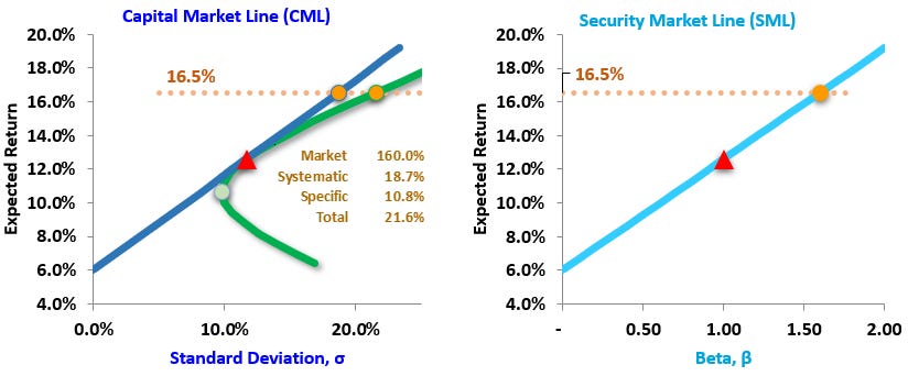
The Market portfolio (the red triangle) has the highest Sharpe ratio. My favorite distinction between the CML and SML is that …
The CML plots only (the most) efficient portfolios, but the SML plots all portfolios (including inefficient portfolios)
First, the SML (on the right) at the orange dot plots an expected return of 16.5% given a beta of 1.60.
Second, the CML (on the left) plots two orange dots on the same horizontal line: both portfolios also have an expected return of 16.5%. The dot on the CML assumes a high-leverage 160% allocation to the Market portfolio. The other dot lies on the two-asset portfolio possibility curve (PPC). Inside the PPC are displayed the risk metrics for this portfolio. The portfolio’s total risk is given by sqrt(18.7%^2 + 10.8%^2) = 21.6%. Systematic risk contributes 18.7% and specific risk contributes 10.8% (or really their squares sum to 21.6%^2).
Both orange dot portfolios in the left plot have the same beta of 1.60. The portfolio on the CML is a mix of the optimal Market portfolio and riskless cash; it is perfectly well-diversified. Only portfolios on the CML are "perfectly" well-diversified such that they contain zero specific risk. The portfolio on the green PPC offers the same expected return (in this case, +16.5%) and it has the same 1.60 beta, but it has additional specific risk. There is a sense in which we can say the portfolios on the green PPC are more diversified as they "get nearer" to the Market Portfolio (which is truly well-diversified and optimal because it has the highest Sharpe ratio, which also means it has zero specific risk). If you are studying for the FRM or CFA, that’s interesting:
Truly “well-diversified” is the unrealistic, optimal state of zero specific risk. Diversification is not a yes/no question. We can measure degrees of diversification in mathematical terms and most portfolios, at best, will be “somewhat” or “almost highly” diversified but—unless it’s a very broad index—manual portfolio constructions invariably will not achieve a “well-diversified” state.
I see two implications with respect to the original question (beta’s relationship to diversification). First, any stock (including a high-beta stock) does not diversify to the extent it adds specific risk. It even appears that the natural convexity says to expect higher specific risk for higher-beta stocks (although I can’t immediately deduce that!).
Second, a portfolio’s beta is conveniently the weighted average of its component betas …
… and the portfolio’s variance is given by:
We can see that adding a high-beta stock will increase the portfolio’s beta (first equation) which increases the portfolio’s volatility (second equation).
So I’d combine the above observation to give the second part of an answer to the question (but of course this is a different beta):
To add more of a high-beta stock is to directly increase the portfolio’s beta (per beta as a simple weighted average) which increases the portfolio’s volatility. Further, unless the portfolio is already well-diversified (aka, zero specific risk), we might expect the high-beta stock to introduce additional idiosyncratic risk.
I hope that’s interesting, thank you for reading!
My actual portfolio is not highly-diversified, it is rather quite concentrated depending on the measure; e.g., sector/industry (I have a lot of tech), size (I’m a bit of a barbell, with a few big companies and a lot of small bets), and to be honest, I don’t even know my portfolio beta although I’d suppose it’s on the high side.
See two-thirds down the transcript here that I used to help me “fact check” this article. The ultimate source for these terms (where I learned them, as applied in Excel) is the FRM P2.T8, specifically Phillipe Jorion’s Value at Risk, 3rd edition. You might notice in the GPT4 transcript that I fact-check my math against Eric Zivot’s Chapter 14 in his Introduction to Computational Finance and Financial Econometrics with R. He’s forgotten more than I know about this (I’ve taken some of his datacamp coursework), and this looks like an excellent reference.
In matrix notation, portfolio variance (0.0225 in this example) is given by x'Σx or w'Σw where x|w is the weights vector. We post-multiply then pre-multiply like this x'(Σx). For this article, I wanted to go down the page (rather than across ), so I transposed the weights from their typical column vector to a row vector. So my x(Σx') in Excel uses =MMULT(C3:E3,MMULT(C6:E8,TRANSPOSE(C3:E3))).
Indeed, +1% to AAPL increases the volatility from 15.00% to 15.2090%. The first derivative is linear so as a linear approximation it’s inexact but very close when for a small change: here the difference is only 0.0006% or 0.061921 basis points.
I don’t think this value represents anything directly meaningful, but I haven’t explored it. It excludes weights so I think it will fail as a rule when the weights are stressed. For example, at very low initial weights APPL becomes a diversifier; inversely, at very high initial weights KO becomes an anti-diversifier.