

What is equity beta?
What is equity beta?
It's just a regression slope; aka, scaled correlation. We should always have questions about a slope coefficient before we trust too much.

The following question was asked this week on the forum:
"Stocks with betas above 1.0 are quite sensitive to systematic risk with low diversification benefit. What does this low diversification benefit mean in the case of a securities? CAPM enables us to measure the expected return of an asset. But what is the relationship between holding a diversified portfolio and the expected return of an asset? The link between beta of an asset and the diversification benefit is a bit confusing."
I like this question1. But I think it’s hard to answer if we aren’t first clear on the definition and meaning of equity beta. Note: this is Part 1 of my response. Part 2 is here.
Beta is a regression slope
Let’s give it a number, for example. What does it mean for a stock to have a beta of 1.380? Beta is the slope of a regression line:
R(i) = α(i) + β(I,M)*R(M) + ε(i). For example, if the beta is 1.380 then:
R(i) = α(i) + 1.380*R(M) + ε(i)
If I wanted to connote a portfolio, maybe I'd use R(P) or R(¶) instead of R(i). But R(i) can refer to a security’s or portfolio’s excess returns. These excess returns could be daily, weekly, or monthly; they can be any periodicity. R(M) is the market’s excess return. This univariate regression symbolizes our hypothesis that the portfolio’s returns are sensitive to the market2.
What’s the regression specifically? It is a regression of the stock’s excess returns (aka, dependent variable) against the market's excess3 returns; aka., independent variable. Most of us do know how to interpret a slope:
For each +/- 1.00% change in the market's return, we might expect +/- 1.38% change in the stock’s return . For example, if the market's excess return is +2.0%, we might expect this security to return +2.76%; but if the market's excess return is -3.0%, we might expect this security to return -4.14%.
In this interpretation, our high-beta stock is very sensitive to the market. If the market jumps, we expect this stock to jump even higher. Conversely, the essence of our high-beta stock is its risk to the downside: if the market drops, we expect this high-beta stock to drop even further. In clinical theory, we expect to pay less today for this risk in the form of a higher discount rate applied to future expectations. Notice how classic theory frames this high-beta stock as riskier (due to its higher sensitivity to the market) and its higher expected return is a function of this risk. To illustrate symbolically, assume the riskless rate is 3.0%, the equity risk premium is 5.0%, and we expect the value of stock will be worth $20.00 in four years:
If the beta is 1.00, the discount rate is 3% + 5%*1.00 = 8.00%, and the stock’s present value is $20.00/1.080^4 = $14.70. Now increase the beta:
If the beta increases to 1.38, the discount rate increases to 3% + 5%*1.38 = 9.90% and the stock’s present value drops to $20.00/1.099^4 = $13.71. Higher risk makes the stock cheaper (i.e., lower present value) which in turn implies a higher expected return.
But if I report to you that a high-beta security has a beta of 1.38, does it prima facie convey great meaning? I don’t think so myself. There are (at least) two things I'd be thinking about:
What exactly are the terms of the regression that generated the beta? There are many questions a data scientist can ask about a regression. For example: We didn’t really regress against the whole “market”, we regressed against an index as a proxy. Which index is the independent variable? Here’s another crucial question: What was the historical window (e.g., three, five, ten years) and periodicity (e.g., daily, monthly) of the returns? When you consider the question of the measurement window, you’ll immediately notice that a stock might have a range of possible betas.
If we use the beta to predict returns, to allocate assets—or as some ex ante input assumption—then we're assuming the past is stable prologue. This is a ginormous assumption. What if the past dynamics no longer apply? What if some regime change renders this historical, statistical artifact a semi-useless quantity? Just because we decided to measure a relationship-thing between two vectors does not imply that thing actually exists.
Beta can be high due to correlation or volatility
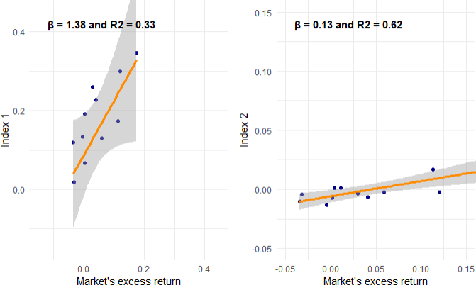
To illustrate that slope is just slope, I simulated two sets of random portfolios against random market returns4. The sample is small, n = 12 months. The blue line plots the linear regression. The shaded grey is a 95% confidence interval per ggplot's default in geom_smooth(method = "lm", se = TRUE).
First set (below): On the left is a high-beta stock (1.38) with a lower R^2. On the right is low-beta stock (0.13) with a high R^2.
Second set (below): Now the high-beta stock (on the left) instead has a very high R^2, but the low-beta stock (on the right) has a very low R^2. I'm just trying to show that a slope (aka, the beta) really wants context before it can tell you something!

What’s my point with these four (above) scatterplots? To show the beta can high but not keenly correlated with the market, and it can be low but highly correlated with the market. My high-beta/low-R2 was generated by amplifying the stock’s volatility. My low-beta/high-R2 was generated by depressing the stock’s volatility but tracking with the index. Meanwhile, the extremely wide confidence interval of the low-beta/low-R2 (lower right) suggest its beta might not even be meaningful; i.e., is that a safe stock or is it just random?
Beta is correlation scaled by cross-volatility
A good thing to know about a regression slope is that it's directly related to the correlation:
β(i,M) = cov(i,M)/σ^2(M) = ρ(i,M) * σ(i)/σ(M), or
ρ(i,M) = β(i,M) * σ(M)/σ(i)
If our 1.38 beta stock has dramatic return volatility of 44% while the market's volatility is only 20% then the implied correlation is given by ρ(i,M) = 1.38 * 20%/44% = 0.6273.
In this way, we can say beta is correlation scaled by cross-volatility5. Or that beta scales a unitless correlation into a unitless beta, but the unitless beta is an informed unitless: 1.38 refers to +1.38 percentage points in the stock’s return per +1.00 percentage point in the market’s return.
Further—and finally!—we can see that a high-beta stock can be explained by either high correlation to the market or/and high volatility (relative to the market’s volatility).
Beta (like correlation) is just a relationship statistic between two vectors
The next thing I'd highlight is underestimated when learning finance: mathematically, both beta and correlation are relationships between any two variables; i.e., return vectors. It happens to be that we are usually referring to the relationship between a security (or portfolio of securities) and some index (as a proxy for the market). But we can regress, or retrieve the correlation between, any two (or more) vectors.
That's why I do not like to write "the beta is 1.38" but rather I try to always write "the beta of the security with respect to the index was 1.38". Correlation is symmetrical: ρ(i,M) = rho(M,i) = 0.6273. Beta is not symmetrical. It would be atypical, but notice that β(M,i) = 0.6273* 20%/44% = 0.285. Not as familiar, but a valid mathematical quantity.
Beta within the portfolio; β(A, ¶ = A+B)
The best way to highlight this general property of beta is to show a two-asset portfolio. I'll assume an equally-weighted (50/50%) portfolio. The volatility of Asset A is 20.0% and the volatility of Asset B is 32.0%. I set their correlation to low at 0.10. Notice (below) how portfolio volatility is lower than the lowest individual asset volatility; i.e., 19.7% is lower than 20%. That's diversification’s superpower in action. An imperfect correlation (< 1.0) enables this superpower. We might even define diversified as a state when correlations are reliably imperfect.
Based on those four assumptions (50% weight, two standard deviations, and correlation), I added some other calculations:

I'll assume you can retrieve the portfolio's volatility of 19.70%. Next are some uncommon calculations. Consider Asset A:
The COV(A, ¶) is the covariance between Asset A and the portfolio that itself includes Asset A. Because here the Portfolio, ¶ = 50%*A + 50%*B, it follows that COV(A, ¶) = COV(A, 50%A + 50%*B) = 50%*σ^2(A) + 50%*COV(A,B)
The marginal volatility, ∂σ/∂A, is the unitless sensitivity of portfolio volatility to the Asset's A weight
The component volatility scales (multiplies) the marginal volatility by the weight; i.e., 0.1178 * 50% = 5.89%. The component volatilities sum to the portfolio volatility.
Beta(A, ¶) is the beta of Asset A with respect to the portfolio (that itself contains Asset A). Because beta is COV(A, ¶)/σ^2(¶), here it is 0.0232/0.197^2 = 0.598.
I wanted to show the beta of an asset with respect to the portfolio, and highlight how it is a different quantity than either the beta of the asset with respect to the market or the beta of the portfolio with respect to the market. Like correlation, beta is just a quantity that summarizes a relationship between two vectors.
Next post
In the next post (Part 2), I promise to try and actually answer the question! Before I do that, I wanted to make sure we are clear what is meant by—and what questions to ask about—a “high beta” stock.
Do you like this question? Maybe you don’t because you think it’s compounding and imperfectly specified. I disagree. I think most good questions are imperfectly specified because they can’t presuppose the answer. The perfectly specified question tends to answer itself. As a teacher, many times my task is to translate the question into its more direct version. But attempts to articulate confusion are noble per se. This question, actually, isn’t even confused. I think it’s almost perfect in its clarity, all five sentences. The assumptions are each correct, and the connection (the question) is almost perfectly identified. To me, it is further good because you can know all of the assumptions, but answering the actual question asked is non-trivial.
In a linear regression (uni- or multivariate), the slope coefficient is something I prefer to call a “sensitivity”. As such, a high-beta stock was highly sensitive to the market’s (or index’s) return over the measurement period. We could also say it’s a measure of association or linear dependence. As you probably know, none of these terms suggest causation. This hypothesis does not strive for causation. Nor do we need causation. We only need the relationship to be useful. If the historical relationship persists—for whatever reasons—it may be useful. In fact, it may be convenient that so much complexity (the complex truth of the actual relationship) is tucked under the rug, in favor of one simple relationship that has some utility.
An excess returns are returns in excess of the risk-free rate. If the risk-free rate is 3.0% and the gross return is 5.5%, then the excess return is +2.5%.
Link to notebook, TBA
This is what I meant in the subtitle that beta is scaled correlation. Of course, this beta is commonly called a measure of systematic risk. Recall that slope is a sensitivity measure. Equity beta is β(i,M) which is sensitivity to the market’s (the system’s) return. So I think that’s a very good fit! Notice that calling beta a measure of “volatility” or “correlation” is incomplete. This CAPM-type beta is the portfolio’s correlation to the market multiplied by the cross-volatility; or, scaled by relative volatility. Hence, to me, the shortest possible definition of this beta is “scaled correlation” or “correlation scaled by relative volatility.”