


Volatility is a model
Being itself unobservable, it cleaves to a subjective model (window and frequency choices). GARCH generalizes EWMA with mean reverting term; both effectively shorten the window via declining weights.

Contents
Volatility as annualized standard deviation
Volatility varies by frequency (periodicity) and window
EWMA assigns more weight to recent returns
GARCH(1,1) generalizes by mean reverting to a long-term variance
The actual returns are non-normal (heavy-tailed) so we want to be careful about unduly imposing normality
Summary
The code for this post is located here at my Quarto data science site.
Last week I introduced value at risk (VaR). As I continue my visualization practice1, it seemed natural to follow up with an introduction to volatility. As an investor and teacher, I'm sometimes humbled and haunted by the idea of volatility. I don’t mean my portfolio’s experience of volatility2. Rather, it’s the way that volatility—a metric at the very foundation of risk, after all—eludes a singular, objective definition. This is because volatility cannot be directly observed: it has no instantaneous existence without a model. Many financial metrics are unobservable, but volatility is uniquely cleaved to its model choice. I also hesitated to write on the topic because it occupies half a shelf on my bookshelf 3 (and years of discussion on the BT forum). My goal here is to show and explain some code I wrote this week, and hopefully in the process, introduce you to volatility.
First, a quick orientation. Say it’s Friday and we’re observing the week’s closing prices for a stock. We notice it closed Wednesday at $10.00, and then closed Thursday at $11.00. I’ll follow Hull’s notation and use u(i-1) to signify Thursday’s daily log return:
Friday’s closing price slipped coincidentally back to $10.00, so Friday’s daily log return, u(i) was -9.53% as given by:
We need two prices over time to inform a return4. Prices are stock measures, while returns are flow measures. A vector of (n) prices inform a vector of (n-1) returns. Volatility is the dispersion of the return vector, so we need at least two returns to get a returns volatility. As above, three end-of-day prices inform two daily log returns, and that’s enough to get a volatility. The standard deviation of {+9.53%, -9.53%} is 9.53%.
The one thing I did (above) that’s different from the Hull text is my explication of Friday’s return as u(i-1, i) simply to remind it’s a “flow over the day” variable. This will later explain the one slight difference in my code (with respect to timing); it seems small but I will tell you these timing issues have been a source of much confusion.
Volatility as annualized (or daily) standard deviation
If we read "an asset's volatility was 17.5%" without further context, we can infer this to mean the annualized standard deviation of historical returns. In this basic definition we’re just using volatility as a synonym for the familiar statistic that captures the dispersion of periodic returns. It's also realistic to refer to a daily volatility; e.g., in my dataset, Nvidia's (NVDA) daily volatility is ~ 2.82%.
Different frequency (periodicity) but same 4-year window
I continue to use the same three stocks as last week: {PG, JPM, NVDA}. My first plot compares their annualized volatility under three different frequencies (aka, periods or periodicity).

After pulling price data from 2010-12-31 (aka, the beginning of 2011), the key function here is sd()
mutate(rolling_sd = rollapply(get(return_col_name),
                              width = window_width,
                              FUN = sd,
                              align = "right", fill = NA))
From the brief documentation, we can see that R’s standard deviation function, sd(), performs the expected calculation to retrieve the sample standard deviation5:
The return, u(i), is a log return and I showed three versions: daily, weekly, and monthly. These are the periods or frequencies. While the plots visualize three different periodicities, all six lines share in common two assumptions:
The window is four years (is why the lines all start exactly 2015-01-01)
Each standard deviation has been annualized.
As this historical volatility is the dispersion of returns, we need to measure some window. I used four years; e.g., that’s only 16 quarters under the least granular periodicity. I annualized per the square root rule; e.g., a daily volatility of 1.0% scales to 1.0% × sqrt(252) = 15.87%, a monthly volatility of 5.0% scales to 5.0% × sqrt(12) = 17.32%. For this sample, I was a little surprised that periodicity isn’t a huge difference.
Update (2023-11-13): Reader Aninda Dutta raised a question based on a keen observation. He wrote,
In the case of SD of all three different companies, the annualized daily SD is more than the annualized weekly SD, which in turn is more than annualized monthly SD.
Does this indicate that the multiplier of sqrt(t) used to scale up SD over a longer period of time, overestimates the longer period SD?
Yes, in fact in does! The square-root-rule is overstating as it scales; scaling assumes i.i.d. returns and consistent over- or under-estimate implicates the independence assumption. This indicates the returns are negatively auto-correlated; aka, the returns are mean-reverting. For example, PG’s average annualized daily SD (see code) is 17.60%. Because this is scaled, we can infer (I’m rounding) the average daily SD is 17.60%/sqrt(252) ≅ 1.11%. I’ll save you the math, but if I assume a negative autocorrelation of -0.179, then scaling this daily 1.11% implies an annualized (but negatively autocorrelated) SD of 14.7%, which is PG’s annualized monthly SD. Put simply, the autocorrelation implied by the {daily = 17.6%, monthly = 14.7%} is about -0.179, according to my back-of-the-envelope6.
Different windows but same daily frequency
Next I held periodicity constant (hovering on daily volatility) while varying the historical window. The window length makes a difference! Notice the jump when Covid hit the market (showing just PG and NVDA, see code for all three).


Using the gt package, I summarized the rolling daily volatilities. NVDA is quite sensitive to the window. Notice how NVDA’s most recent volatility does not dampen with a longer window, as you might expect.

Exponentially weighted moving average (EWMA)
What is the point of estimating today’s volatility (or the most recent volatility; e.g., NVDA’s 2.76% or 2.47% or 3.25% or 3.63%)? Probably the point is to estimate a current volatility and/or to predict a forward volatility. If that is the case, does it bug you that when estimating a 250- or 500-day volatility, we’re assigning the same weight to distant returns as yesterday’s return? Shouldn’t we give yesterday’s return more weight?
Enter the versatile ARCH(m) model as given by:
Let’s make two simplifying assumptions in order to retrieve a special case:
Let’s assume there is no long-run variance, V(L), such that we drop the first term
Let’s assume the weights, α(i), decline exponentially
This simplifies to the EMWA variance as given by …
and executed in my code with the loop:
ewma_var[i] <- lambda * ewma_var[i-1] + (1 - lambda) * returns[i]^2 Lambda, λ, is the smoothing parameter. If λ = 0.940, then the most recent (aka, yesterday’s) squared-return’s weight is 1 - 0.94 = 6.0%. What about the day before that? It’s weight is 6.0% * 0.94 = 5.64%. And the day before that gets a weight of 5.64% * 0.94 ~= 5.30%. Lambda is the ratio of consecutive weights. The older the squared-return, the less weight it contributes to the estimate. A lower lambda is less smooth and more reactive. You might observe that this effectively shortens the window.
Next I plotted EWMA against the (prior) rolling standard deviation; I used a typical λ = 0.94 parameter. Even for a seemingly high smoothing parameter, this EWMA is reactive in comparison:

My rolling volatility above (rolling_sd) has a 4 year (1,000 day window). The EWMA has only a 250 day window, but that’s longer than I need. With λ = 0.94, the 250th return has virtually no weight; it’s weight is given by (1-λ)*λ^(n-1) or 6%*0.94^249 = 0.0000012%. In fact, the most recent 38 days account for >90% of the cumulative weight.
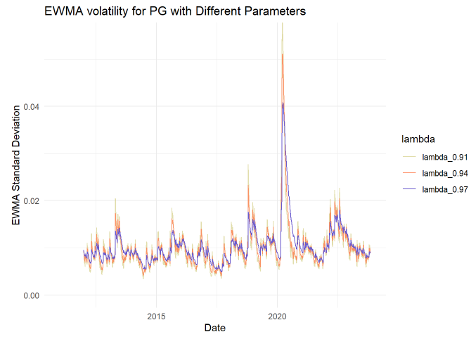
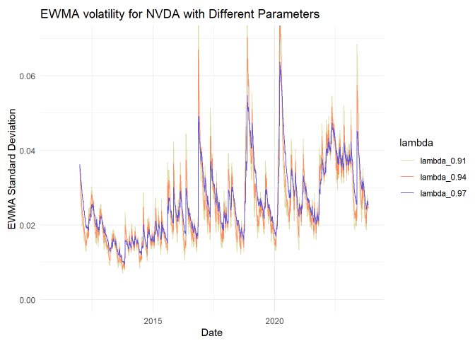
I was curious to see the influence of varying the lambda parameter, in this case the comparison set is λ = {0.91, 0.94 and 0.97}.
GARCH (1,1)
Finally, we will reintroduce the first term, γ*V(L), that we dropped for EWMA. Setting aside theory, we’re generalizing from EWMA to GARCH(1,1):
EMWA’s smoothing parameter, λ, maps to beta, β
The reactive weight, (1-λ), maps to alpha, α
EWMA’s two weights sum to 1.0: λ +(1-λ) = 1.0. But GARCH adds a weight (“generalizes”) to the long-run (aka, unconditional) variance. That weight is gamma, γ, so such that GARCH’s three weights sum to 1.0 = α + β +γ .
This seems like an elegant way to estimate today’s volatility: prior (squared) returns are incorporated but with exponentially decreasing weights (beta); the recent (squared) return is directly weighed (alpha); and the series is gravitationally pulled toward a long-run value.
Fitting the parameters
I used the rugarch package. Frankly, I have not used it before (in the FRM, we tended to fit the parameters with MLE in Excel), but the results look plausible:

You might notice that I inferred the long-run volatility with …
LR_vol = sqrt(omega / (1 - alpha1 - beta1))…. because the first term omega is the product of the weight (γ) and the long-run variance, V(L); i.e., ω = γ*V(L) such that V(L) = ω/γ = ω/(1 - α - β).
Rolling GARCH(1,1) for {PG, JPM, NVDA}
To plot rolling GARCH for my three stocks, my function calculate_garch_variance() has a simple loop that computes garch_var[i] over the length of the daily window given by W.daily (1,000 trading days = 4 years).
calculate_garch_variance <- function(returns, alpha, beta, gamma, W) {
    long_run_variance <- var(returns[1:W], na.rm = TRUE)
    omega <- gamma * long_run_variance
    garch_var <- rep(NA, length(returns))
    garch_var[W] <- var(returns[1:W])  # Initialize the first GARCH variance

    for (i in (W+1):length(returns)) {
        garch_var[i] <- omega + alpha * returns[i]^2 + beta * garch_var[i-1]
    }

    return(garch_var)
}
To visualize, I used the same {α, β} parameters for all three stocks:
garch_sd: α = 0.12, β = 0.78, γ = 0.10 and specific V(L)
garch_sd_mr: α = 0.03, β = 0.83, γ = 0.14 and specific V(L)
The point of garch_sd_mr (colored orange) is to illustrate a version where a “pull toward the mean” is exaggerated, and the long-run weight is very high at γ = 14%.

None of the returns are nearly normal
The last thing I did for this introduction is just a reminder. Sometimes you’ll see somebody calculate volatility and subsequently apply a normal deviate; e.g., NVDA has an overall standard deviation of 2.8227% such that somebody might suggest their 95% one-day VaR is given by 2.8227% * 1.655 ~= 4.64%. But that’s imposing normality! Almost every time we sample stock returns, we find them to be heavy-tailed, and often skewed as well.

At the bottom of my code, you can observe sample moments for each of the stocks
In regard to skew, PG and JPM exhibit negative skew. For stocks, this negative skew is typical: while most of the daily changes are small and often positive, there are large negative returns that occur more often than you’d expect if the distribution were normal.
In regard to kurtosis, all three stocks exhibit heavy tails with kurtosis values of {PG = 14.7342, JPM = 13.3437, NVDA = 10.6039}.

Summary
I said “volatility is model” to emphasize that we subjectively infer volatility by choosing a model7. Volatility is typically annualized standard deviation. The drawback here is that a realistic sample reaches back to give distant returns-squared the same weight as recent returns; it is an equally-weighted approach. When measuring volatility, we want to be mindful of our choice(s) with respect to frequency (e.g., daily returns) and the historical window.
An interesting finding in my sample: window makes a difference, but frequency not so much.
EWMA improves on this by decreasing the weights (in a constant ratio given by λ) and further the series formula reduces to an elegant two-term expression. GARCH(1,1) generalizes on EWMA by adding a term that assigns some weight (γ) to the long-run variance toward which the series mean reverts. By virtue of decreasing weights, both EWMA and GARCH(1,1) effectively shorten the window.
P.S. GPT-4 did help me write some of the code. Specifically, TBA.
I’ve practiced ggplot for years, enamored by the tidyverse. The grammar of graphics is supremely elegant. I also think data visualization is an increasing important skill. As with my VaR article, most of the time that I spent on this code + article was spent on tweaking the visualizations. In particular, the color palette is deliberate. There is so much to learn!
My investing style—which requires some patience—is basically indifferent to daily volatility. In fact, I’d gladly accept compensation for short term volatility.
My book recommendations for volatility are these three (my notation follows John Hull because his text is the most accessible; but Stephen Taylor has the most technical treatment).
Alexander, Carol. Market Risk Analysis. 2 : Quantitative Methods in Finance : Practical Financial Econometrics. Wiley, 2008.
Hull, John. Options, Futures, and Other Derivatives. Pearson Education Limited, 2022.
Taylor, Stephen J. Asset Price Dynamics, Volatility, and Prediction. Princeton University Press, 2011.
Log (aka, continuously compounded or geometric) returns are conveniently time additive. They approximate simple (aka, arithmetic or holding period) returns which are cross-sectionally additive. For daily periods, the difference tends not to matter. It might for the other periodicities.
The (n-1) divisor suggests a sample standard deviation, but it would also be okay to divide by (n). They are different estimators (unbiased variance versus MLE). Setting aside estimator properties, to me it’s easiest to just think of (n-1) generating a slightly more conservative (i.e., larger) estimate.
The more significant decision is whether to include the mean (this is called the mean deviation form), or to exclude the mean (I call this the zero-mean form). You’ll notice this rolling standard deviation is a technically “proper” standard deviation because it uses the mean deviation form; i.e., it includes the mean. In my EMWA and GARCH(1,1) code, you will notice that I simply square the return: they are zero-mean form. This is a simplifying convenience. However, the difference can matter at supra-daily frequencies. Here is a way to think about it. What if the period returns were somehow magically {-5%, -5%, -5%, …. }. What volatility would you expect/prefer?
Because my example scales both daily and monthly returns, I think the mean reversion is (mathematically) divided between the two dynamics; i.e., my example attributes the entire reversion to violations of i.i.d. daily returns. But I don’t think that changes the directional finding that this pattern indicates mean reversion in returns.
Link to last year’s post at https://www.linkedin.com/posts/bionicturtle_option-vega-frm-t4-17-activity-6926568087676743681-wSBY