
Value at Risk (VaR)
Historical and bootstrap simulation with {PG + JPM + NVDA} portfolio. Monte Carlo and parametric illustrations. VaR is just a distributional quantile.

Contents:
Basic historical simulation (HS)
Bootstrap HS
Monte Carlo
Parametric (Basic = normal, arithmetic i.i.d. returns)
Some technical notes
This post discusses my code notebook that’s located here at my data science Quarto site called finedtech.io. I wanted to visualize an introduction to value at risk (VaR). As was the case with my recent posts on linear and logistic regressions, the visualizations took much more time than the wrangling and computation.
If you are new to the topic, the key idea is simple:
VaR is just the quantile of a financially-predictive probability distribution. As such, it’s like the median (0.50 quantile) except it’s a lower quantile—e.g., 0.050 or 0.010 or 0.0010—because it concerns our potential unexpected losses
That’s the easy part: if we can specify a plausible probability distribution, VaR is just a descriptive statistic that we retrieve from the distribution. The hard part is specifying a realistic distribution. Specification is hard because VaR is naturally the worst expected loss—with some confidence over some horizon—of a future distribution. This is a distinction that might be easy to gloss over, so I’m going to emphasize it again:
In finance, much of the analyst’s work concerns their effort to discern the present value of a thing (an asset, portfolio, or position) and this is a noble exercise in precision. Risk measurement is a different practice: we are trying to imagine and quantify future possibilities. This endeavor cannot be precise; indeed, we are satisfied with useful approximations. VaR belongs to future and not the future’s expected (aka, mean) value but its other moments. VaR cares about the loss tail’s shape and weight (and its wide standard error). Although we are mathematically rigorous, we can’t forget it’s an operation on the unknowable future. Ergo, specification of the future possible distribution must be a hard task.1
In the broadest terms, we can choose either a non-parametric or parametric approach2. Non-parametric let’s the data speak3 without imposing an analytical probability function. If we are going to rely on data, we either use historical data or manufacture data. Consequently, the non-parametric approaches divide broadly into historical simulation versus Monte Carlo simulation. Let me show you those first.
Basic historical simulation (HS)
You can see my code chunk retrieves periodic (daily | monthly) log returns for three stocks over a recent ten-year period: Procter & Gamble (PG), JPMorgan Chase (JPM), and NVIDIA Corp (NVDA). I used tq_transmute() from the tidyquant package4, which wraps quantmod’s periodReturns to make it easy:
all_returns_monthly <- mult_stocks |>
    group_by(symbol) |>
    tq_transmute(select     = adjusted,
                 mutate_fun = periodReturn,
                 period     = "monthly",
                 type       = "log")
To retrieve the 95.0% VaR via basic historical simulation is to retrieve the 0.050 quantile() of the dataset:
quantiles_monthly <- all_returns_monthly |> group_by(symbol) |> reframe(quantiles = quantile(monthly.returns, probs = c(0.05, 0.95)))I had more fun plotting the implied densities (in lieu of histograms). The respective 95% VaRs are plotted as dashed lines (see below). The monthly log returns turned out to be interesting. If you owned NVDA, you had the prospect of higher returns, but its one-month 95.0% basic HS VaR is ~20.2%.
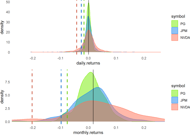
How do we interpret that in a sentence? If history is predictive, we’d say:
We’re 95% confident that our worst loss (in the NVDA position) over a one-month horizon will not exceed 20.2%. Equivalently, we do expect the one-month loss to exceed 20.2% once every 20 months (5% of the time), and further, our VaR measure doesn’t say by how much.
Bootstrap historical simulation (HS)
An interesting enhancement is the bootstrap HS. The key idea here is sampling (the historical return vector) with replacement. In my code, the key function is:
# Simulate one forward month
simulate_one_month <- function(portfolio, historical_returns_wide) {
# Randomly sample one month's returns (with replacement)
sampled_returns <- historical_returns_wide |>
sample_n(1, replace = TRUE) |> select(-date)
# Apply the sampled log returns to the current portfolio value
updated_portfolio <- portfolio * exp(sampled_returns)
# FOR TESTING: print(sampled_returns[1,]); print(updated_portfolio[1,])
return(updated_portfolio)
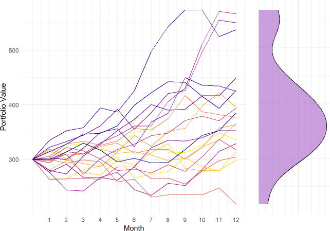
}In this simulation, I start today with $100 invested in each of PG, JPM, and NVDA so the initial portfolio value is $300. Then I want to simulate the portfolio forward one month. To do this, I randomly sampled the log returns from one of the months in the historical window—which returns a vector of three sampled_returns—and grow the portfolio by applying those returns via element-wise multiplication: portfolio * exp(sampled_returns). By repeating this eleven more times, I’ve simulated the portfolio over 12 months, to the end of the hypothetical year. That’s one path (aka, trial). My simulation only plotted 20 trials. Then I plotted (sideways) the implied density distribution of the final values.
Monte Carlo
Monte Carlo simulation is powerful and flexible. But I’m just going to show here the most common equity simulation, which is the lognormal property of stock prices (aka, Geometric Brownian motion, GBM). The key line in my MCS code is the following line, where Z is random standard normal:
prices[t] <- prices[t-1]*exp((mu -0.5*sigma^2)*dt +sigma*sqrt(dt)*Z)The plot (below) visualizes 20 trials where each trial is 50 weeks (periods).
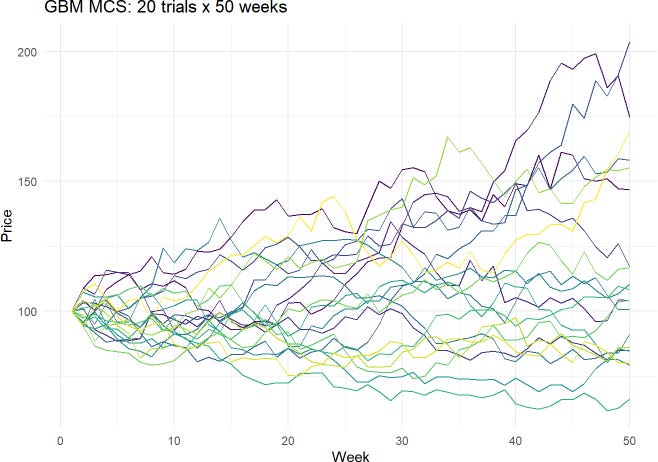
This simulation generates a set of final end-of-horizon prices (i.e., 20 different stock prices at the end of 50 weeks) which itself is a distribution. From that distribution, we can retrieve an X% quantile; aka, an X% VaR.
Parametric (Basic = normal, arithmetic i.i.d. returns)
I’m going to use the normal distribution to introduce a super simple parametric VaR, but please note there’s a common misconception that parametric VaR assumes normality. It does not! We can fit any distribution. Nevertheless, I’ll use a normal here due to its convenience and familiarity5. Because I assumed a normal distribution, my parametric VaR code chunk only requires two distributional assumptions: mean, μ, of +9.0% per annum with volatility, σ, of 20.0%. To retrieve a VaR, we need to make two “design decisions:” what’s the confidence level, and what’s the horizon? I looked for a 12-week, 95.0% VaR with this command:
z_score <- qnorm(confidence_level)
VaR <- (-mu + sigma * z_score) * investment_value
The distribution is plotted below. Notice the VaR of $13.726 is our worst expected loss (with 95% confidence) over the 12-week horizon relative to our initial position of $100.
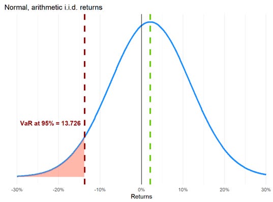
Specifically,
At the end of the 12-week horizon, the position’s expected future value is $100 * (1 + 9%*12/52) = $102.077 due to its expected gain (aka, drift) of 9.0% per annum
The relative VaR is $15.803 because that is the worst expected loss relative to the expected future value of $102.077
The difference between $102.077 and $15.803 is $86.274. If the stock drifts up as expected (to $102.077 in the future) but, relative to this level, exhibits its worst expected loss (of $15.803), then it will fall to $86.274
A drop to $86.274 is a loss of $13.726 from the initial value of $100.00, such that $13.276 is called the absolute VaR. This absolute VaR ($13.726) is less than relative VaR ($15.803) by the amount of the drift ($2.077).
My VaR calculations here assumes the arithmetic returns are normal; i.e., S(t)/S(t-1) - 1 is an arithmetic (aka, simple) return. Alternatively, if I had assumed the log returns, ln[S(t)/S(t-1)], are normal then we’d compute a lognormal VaR.
The relative VaR excludes the drift; if the drift is zero, they match. The absolute VaR is a return-adjusted risk measure (the positive drift offsets the negative shock), and is generally the superior form.
Some technical notes
We’ve visualized all three major approaches to value at risk (VaR): historical simulation (basic or bootstrap), Monte Carlo simulation and parametric. Historical simulation (HS) is the most popular, and keep in mind: HS has many variations that we did not illustrate.
Here are some additional nuances:
I scaled VaR per the square root rule which, by definition, assumes variance scales with time. For example, if the one-day volatility is 1.0%, then the 10-day volatility is 1.0%*sqrt(10) = 3.162%. The key, unrealistic requirement (aka, assumption) of such scaling is that the returns are independent and identically distributed (i.i.d.).
Like the simulation approaches, the parametric approach is an umbrella that contains many model variations. The most common might be delta-normal VaR (aka, variance-covariance VaR) which assumes the risk factors are multivariate normal and their dependence can be specified with a correlation/covariance matrix. However, that’s just the most convenient among many alternatives. VaR does not require normality, it only requires a plausible specification of future distribution(s).
If we do assume the normal distribution, then we can think of VaR merely as scaled volatility. In terms of Excel functions, the familiar deviates are =NORM.S.INV(95%) = 1.645 and NORM.S.INV(99%) = 2.326.
Among the technical weaknesses of VaR, perhaps the most relevant are:
As a quantile, VaR conveys no information about the extremity of the potential loss. For example, a portfolio’s one-day 95.0% VaR of $1.0 million tells us to expect a mark-to-market loss in excess of $1.0 million dollars once every twenty days, but it does not tell us the expected magnitude of that loss! Maybe it’s -$1.5 million. Maybe it’s $5.9 million
VaR is not coherent: counterintuitively, it can abruptly increase as positions aggregate; i.e., it can confusingly contradict our expectations about the benefits of diversification. On the other hand, expected shortfall (ES) is coherent.
Certain quantiles in a discrete distribution (generally the non-parametric) have multiple VaRs when the quantile falls “in the crack between” two bins (is how I think about it). For example, if the window is 100 days, then for the 95.0% VaR basic historical simulation can retrieve the sixth-worst loss, the fifth-worst loss, or an interpolation. Consequently, when the distribution is discrete, VaR can be ambiguous. However, ES is never ambiguous (as a conditional average, there is always only one ES answer to a given ES question, so to speak).
I hope that is interesting and helpful! Thank you for reading.
If you accept the premise, I’ll go further: valuation exercises that discount future values (e.g., earnings, cash flows) depend on future value estimates. Therefore, risk is antecedent to valuation: we cannot discern the present value of a risky asset (e.g., a share in a publicly traded company) unless and until we have some measure of its risk. In practice, our greater fluency with approximate future risks should contribute to more precise present valuations.
These are broad categories. Some of the most interesting refinements are semi-parametric approaches; e.g., we can parametrically weight historical returns, giving greater weights to more recent returns.
My favorite technical (mathematical) text remains Kevin Dowd’s Measuring Market Risk (2nd Edition). As it has been assigned in the FRM for ~ 15 years, much of my own mastery is based on this book.
The primary author of tidyquant is Matt Dancho, who is the incredibly successful and prolific founder/CEO of Business Science. Definitely go here to learn more data science!
It’s also super convenient to simulate a multivariate normal distribution with a correlation/covariance structure. But you can inversely transform random standard normals into other distributions. See my recent post on the logistic regression for an illustration of the simdata package, where random normal risk factors are inversely transformed into various distributions.