

Future values are the focus of risk measurement
Future values are the focus of risk measurement
Chapter 3: An Introduction to Quantitative Finance for Risk Management

📗 The 2-minute version 📗
Risk measurement is satisfied with imprecise estimates of the tail (and variance, skew, kurtosis) in a future distribution. This agenda interrogates the methodology of our future projections and our selection of discount rate(s). Most of the traditional approaches have drawbacks (well, prediction is hard). Trees incorporate volatility and path-dependence. Risk aversion introduces subjectivity which is important because individuals have different preferences and different portfolios. Simulations are the probably the best approach given the agenda of risk measurement (and therefore risk management)
Contents
Introduction
The discount rate is a bridge between present (PV) and future value (FV)
Risk-neutral valuation is elegant but limited
The discount rate as a function of risk and required return
Introducing uncertainty with random walk (binomial tree) and volatility
Risk aversion introduces subjectivity (including personal portfolio)
Simulation (or stressing the inputs) to create future distributions
Conclusion
This series introduces quantitative finance for risk management. Previously, I explained Present Value (PV) and The Law of One Price, but I have yet to introduce anything particular to risk. Now we reach that fork in the road. We'll ask a question that shifts us away from a traditional path (aka, valuation) and toward an emergent path (risk measurement)1. The question is, How does risk measurement differ from traditional valuation?
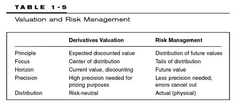
Many years ago—when I was learning risk, long before I taught any risk but just after I'd earned the CFA charter—I scanned a small table2 by Philip Jorion in his classic book, Value at Risk. The table's simple distinction inspired me, and it was permanently etched in my long-term memory. Here is my own re-interpretation of his table:
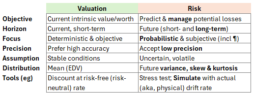
I’d highlight three features of risk measurement (the right-hand column above): we accept low precision; we are obsessed with the future tail (i.e., the distribution’s variance, skew and kurtosis) rather than its mean; and our agenda likely favors numerical simulations over analytical solutions. A maxim taught to new learners in risk is something like:
“We should try to find our ‘unknown unknowns’—a difficult task by definition—but among the knowns, our quantitative mission is to translate qualitative uncertainties, also known as Knightian uncertainty3, into quantifiable risks, ideally in the form of a future probability distribution." —
Me, paraphrasing what many authors and teachers have already said about risk measurement. It is such a pedagogical cliché that I forget to ask if it’s true.
The discount rate is a bridge between present (PV) and future value (FV)
Asset pricing builds a bridge between anticipated future values (or cash flows or earnings streams) and the present. In symbols:
PV = f[E(F1, F2, …)]
That is, the single present value is some function of the estimates of multiple future values across different time horizons. We predict future values (F1, F2, …) and discount them to their present value (P) via a discount rate or expected discounted value (EDV) function. I’ll use F instead of FV, and P instead of PV4.
Among the first things a finance student learns is the zero-coupon relationship between the present and the future, as given in discrete terms by its general form (where k is the number of periods in a year; aka, compound frequency):
As k increases above monthly (k = 12), weekly (k = 52), and daily (k = 250 or 252), k tends towards infinity, k → ∞, and we get the continuous instance:
I love the elegance of P = F*exp(-rT) because it is a compact package of four existential variables. The present value, P, discounts the future, F, continuously at a rate, r, over the horizon, T. This expression is the most primitive tool in the financier’s toolbox.
About the present value, P, there is a distinction between a model (aka, theoretical) price and a market (aka, traded, observed) price. We calculate model prices, but we don't actually expect them to match market prices5. Or we may fit our model to market prices, which effectively treats the market price as an input; e.g., option implied volatility, arbitrage-free term structure model. The horizon, T, is often known or specified.
Of course, the two challenging variables are the future value and the discount rate. By future value(s), I am referring to a series of expected future values, E(F1 @ t1, F2, @ t2) where t1, t2 are future points in time. Future value is a vector that captures an expectation; for example, a vector of expected dividends. In some cases, we can reasonably estimate the future value vector (although if we are honest, the vector is probably itself random or fuzzy). Our biggest problem sometimes is calibrating the discount rate. The longer the horizon, the more the discount rate matters.
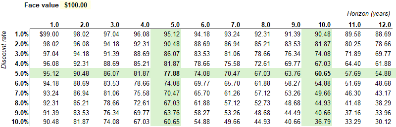
Here is simple way to think about the effects of the horizon and the discount rate. The matrix below assumes a $100 face zero-coupon bond. If its maturity is 5 years while the continuous yield6 is 5.0%, its theoretical price is $100*exp(-5%*5) = $77.88; while the 10-year bond price is $100*exp(-5%*10) = $60.65.
Because this a continuous-yield zero, the sensitivities are super elegant:
∂P/∂r = -T*P ⇒ as a % of P ⇒ ∂P/∂r * 1/P = -T
∂P/∂T = -r*P ⇒ as a % of P ⇒ ∂P/∂T * 1/P = -r
Yield sensitivity is a function of the term and vice-versa. The 10-year term, 5% yield bond has a current price of $60.65. Its sensitivity to the yield (aka, duration) is 10 years: if the yield drops by 1% to 4%, we expect a 10% increase in the price. Its sensitivity to the term is 5%: if the term drops by 1 year to 9 years, we expect a 5% increase in the price7.
To recap: the market price might be observable, but our model's price is a function of an uncertain future value vector and our selection—which may seem like an arbitrary decision—of a justifiable discount rate. How do we mathematically cope with this uncertainty? The common ways include:
Some justify the risk-free rate via risk-neutral valuation. At least it’s observable and objective, probably!
Build up a required rate of return that aspires to account for all risks. (And perhaps translate our expectations into certainty-equivalents for purposes of self-checking.)
Attempt pseudo-realism by constructing a binomial tree
Include a risk-aversion coefficient (or otherwise formalize the risk-adjusted expectations).
Simulate the variables with explicitly numerical (as opposed to analytical) approaches.
Risk-neutral valuation is elegant but limited
The challenge is how to calibrate the discount rate. Quantitative finance offers an elegant answer: just use the risk-free rate! If that doesn't feel satisfying to you, I do empathize. Below is my rendering of a classic binomial concept8. My assumption is a one-month call option with a strike price of $52 while the stock price is $50 and the risk-free rate is 5%, i.e., S = $50, K = $52, T = 1/12 years, and Rf rate = 5%. By matching volatility to the up and down jumps, we can assume the stock will jump up to $55.48 or down to $45.06.
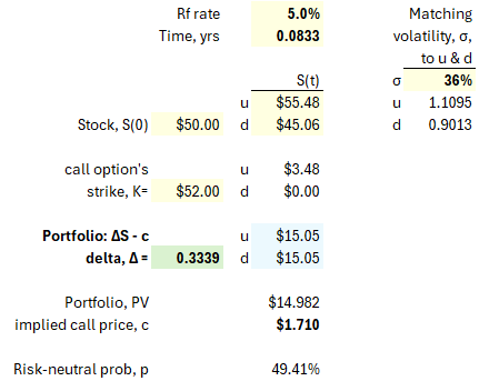
The key calculation here is the option's delta, Δ = [c(u) - c(d)] / [S(u) - S(d)] = 3.48 / (55.48 - 45.06) = 0.3339. Why? Because the portfolio of (short one call option plus long a Δ fraction of one share) is a riskless portfolio with a future payoff of $15.05 regardless of whether the jump is up or down. If the payoff is certain, we can discount it to the present using the riskless rate: its present value is $15.05 / (1 + 5%/12) = $14.982. Therefore, the option's value must be $1.710.
This work similarly for options on bonds. It’s worth studying if you are a serious finance student, but not too much otherwise. The magic is that we can price the derivative without regard to anybody’s risk aversion or risk preferences: the price must be accurate because it is the cost of a package that replicates the derivative’s payoff under any up/down jump scenario! We do not live in a “risk-neutral” world, but we get to apply the results of this imaginary world. Here is an easier way to think about the theory: today’s asset price incorporates both expected future returns and the discount rate. If the asset is riskier, a higher discount rate offsets higher expected returns.
The problem with risk-neutral valuation is that it only applies to derivatives.
The discount rate as a function of risk and required return
The most common approach is to use a discount rate that presumes to reflect the riskiness of future cash flows (or future values). Let's say that today you can purchase a riskless bond that will be redeemed for $100 at the end of one year9. If the riskfree rate is 5%, you are willing to pay $100/1.05 = $95.24.
However, let's now make a more realistic assumption that the bond has some risk of default; it is a risky bond. Your required rate of return will reasonably be higher than 5%. In this case, maybe your discount rate is 8%, such that you are only willing to pay $100/1.08 = $92.59. We might say the risk premium (3% in this example) is compensation for bearing the default risk. In fact, if we assume no recovery (if the recovery rate is 0% then the loss given default is 100%), then the spread approximates the default probability. As such, the 3% spread is compensation for the bond’s default probability of 3%.10
To build up the discount rate is to apply both science and art. It can feel like constructing a loaf of bread by adding slices in sequence. As we are able to somehow articulate additional risks, we add them to the discount rate! The world’s expert on this topic (i.e., cost of capital as an input into discounted cash flows) might be Aswath Damodaran; here is his recent post on the role of risk in the cost of capital. His post last year (The Price of Risk) is as good as you’ll ever read on the construction of the equity risk premium (ERP) that informs the discount rate (i.e., Expected Return = Riskfree rate + Risk Premium) in the equities asset class.
The capital asset pricing model (CAPM) is intuitively convenient, but its basic version specifies only a single common factor (the equity risk premium or market risk premium). Consequently, there are multi-factor extensions that presume to be more realistic. We can generalize from the CAPM to the APT/multifactor model11 as given by:
The above expression reflects a really core idea in finance: risk determines expected returns because risk premiums are compensation for exposure to risk factors12. As you add exposure to additional risk factors, your expected return should increase.
Practitioners and scholars have studied and tested many factors. If we want to critique this model, we might notice:
It's a linear model that enables a convenient point estimate of the expected return.
We can't realistically expect the factors and sensitivities to remain static over time.
Illustration of CAPM and certainty-equivalent cashflows
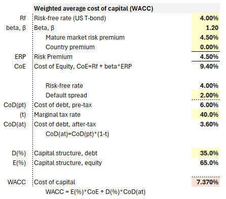
Let's look at an example below. This hypothetical firm's cost of equity (CoE) is built-up as a function of a market risk premium (although the country premium is zero). This contributes to a weighted average cost of capital (WACC) of 7.370%.
We can imagine a project that requires an expected initial investment of $1,000 followed by another $400 in the first year. Subsequently, we expect the project to generate cash flows in the second through fifth years, {0, +300, +700, +1200}, with an expected terminal value of $1,500. In the left panel (below), these expected cash flows are discounted at the WACC of 7.370%.
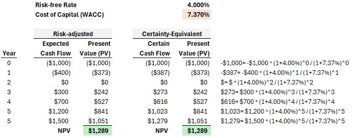
In the right panel (above), I've translated the expected cash flows into their certainty equivalents (CEs), then discounted those CEs at the risk-free rate. By definition, we get the same net present value. The project does have risks. In the typical approach, we increase the discount rate to reflect our estimate of risk. More risk warrants a higher discount rate. The CE approach is a translation that asks us to think about our assumption (the discount rate) in a different way: if our discount rate is sufficiently high, then we should be virtually certain we can achieve the "certain" cash flows. The "certain" cash flows are discounted at the risk-free rate. Put another way, if the CE cash flows accurately reflect lower bounds on future cash flows (with confidence approaching certainty), then we've sort of validated the discount rate. If the CE cash flows do not represent confident lower bounds, then we've underestimated the discount rate.
Introducing uncertainty with random walk (binomial tree) and volatility
A popular way to formally introduce volatility is with a binomial tree. Previously, I illustrated a one-step tree, but a typical binomial tree has many steps. The binomial tree is popular in option pricing. Below I've illustrated a simple two-step tree, but you can imagine its extension to many steps. We do require a logic that informs the up/down jumps and their probabilities. In this illustration, I use a volatility assumption of 30% per annum to inform the three parameters (u, d, and p) required to grow the tree: up, down and probability. Two mini-trees are displayed: the stock price tree (in green) and the corresponding, implied option value tree (in blue), where I've assumed a strike price of $22.00 when the initial stock price is $20.00.
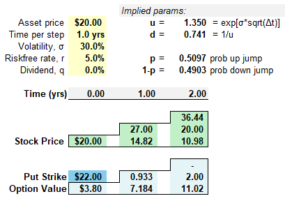
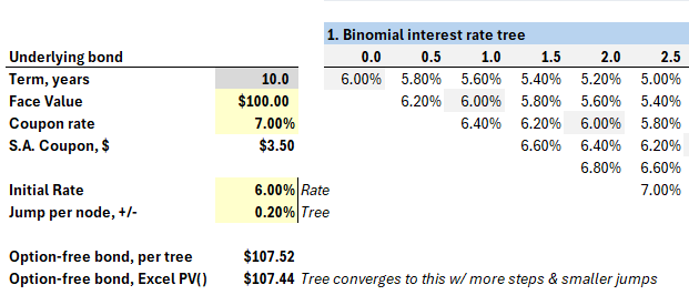
The exhibit above has two trees: one for the stock price, and a mirror tree for the implied option price. Typically we “grow out” the underlying asset, then backwardly induce the option’s value. We can build a tree for any variable. For stock options, we naturally build a tree for the underlying stock price. In the fixed income asset class, the key risk factor is an interest rate (so the tree builds out an interest rate such as yield or future short-term rates) . There exists a large cluster of term structure models—from simple to sophisticated—that can inform the interest rate tree. For example, the interest rate can be mean reverting, and should not be able to go below zero. Below is a snippet of my option-adjusted spread (OAS) model with an unrealistically naïve assumption: at each node, the interest rate jumps up or down by 20 basis points.
The binomial is highly intuitive and overcomes the mistake of estimating the future as a single path (e.g., it is very good at valuation of path-dependent bonds or options), but its salient drawbacks include:
Because it’s an intuitive tree where the first node branches into two nodes that recombine into three nodes (rather than four), it remains a somewhat simple model. Adding realism appropriately complicates the model but also increases parameter sensitivity and model risk.
It’s a natural use case for Excel (and surely that’s were the majority of binomial models currently live!) but Excel implementations of the binomial—as they are not closed form solutions—are unnatural for sensitivity analysis. You can claim otherwise, but I wish I had a nickel for every binomial model that I’ve opened in Excel that contained errors due to the complexity.
Risk aversion introduces subjectivity (including personal portfolio)
For the sake of introductory, academic completeness, I want to briefly mention the academic approach that defines a utility curve as a function of a risk aversion coefficient. Here is the simplest utility function:
In the above function, the expected return is penalized for the anticipated volatility endured to achieve it. By penalizing return with a risk factor, this utility function is similar to the class of ex ante risk-adjusted performance measures (RAPMs). Careful readers will note that U(i) and A(i) have subscripts: this reflects that each individual investor has their own risk aversion coefficient and, therefore, their own utility function. The most popular RAPM is the Sharpe ratio13.
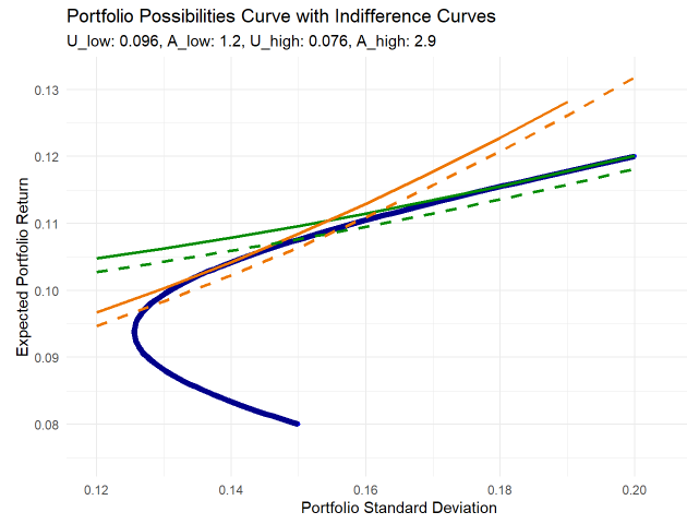
Below is my plot of two utility curves and their tangency to a classic portfolio possibilities curve (PPC). The code for this plot is located on my data science blog here. In this case, the PPC (blue curve) plots a two-asset portfolio where the first lower-return asset has an expected return of 8% with volatility of 15% and the second higher-return asset has expected return of 12% with volatility of 20%; their correlation is 0.10. You can see the endpoints at {σ2 = 0.15, E_r2 = 0.08} and {σ1 = 0.20, E_r1 = 0.12}. Before the indifference curves are introduced, the upper segment of the PPC defines a risk/reward tradeoff for an investor.
There are two sets of indifference curve, green and yellow; a single indifference curve has the same utility at every point.
The investor with high risk aversion (i.e., yellow indifference curves) has the higher aversion coefficient, A = 2.9.
The investor with low risk aversion (i.e., green indifference curves) has the lower aversion coefficient, A = 1.2.
The more risk averse investor (A = 2.9) maximizes her utility at the yellow line’s tangency point, where her utility is 0.96. The less risk averse investor (A = 1.2) maximizes her utility at the green line’s tangency point, where her utility is 0.076. As we might expect, the less risk averse investor’s optimal portfolio allocates more to the riskier of the two assets.
The risk-adjusted utility function introduced subjectivity
While indifference curves (i.e., points with equivalent utility) might introduce us to a useful theoretical framework, they impose many practical challenges14. Ultimately, this approach embeds many strict assumptions.
However, the key achievement in this point of our tour of approaches is that we have formally introduced, and incorporated, the individual investor’s attitude toward risk (A is called a risk aversion coefficient but we might even call it a risk appetite coefficient). Much of the the traditional theory—including modern portfolio theory (MPT)—is essentially objective because it assumes homogenous expectations: all investors have equivalent views on each asset’s returns, volatility, and the correlation matrix. We cannot ignore what I am calling subjective views for at least two reasons:
Each individual has a different risk appetite and tolerance
Each individual has a different portfolio and portfolio perspective. This is not just theoretical, this is incredibly practical. A wealthy individual can, in extremis, make angel investments that would be unsuitable to most people. A young person can afford to concentrate in ways that would be unsuitable to somebody nearing retirement. And so on.
Simulation (or stressing the inputs) to create future distributions
Finance is applied math. There is a distinction between analytical and numerical procedures. Analytical approaches utilize a function. If we use the Black-Scholes Merton (BSM) model to price an option, we are using an analytical approach because it has an elegant formula. Generally, analytical approaches offer the advantage of convenience at the cost of over-simplification. At some point in our use case, we may need to employ a numerical procedure. Finance has seen a shift toward simulation-based approaches in recent decades.
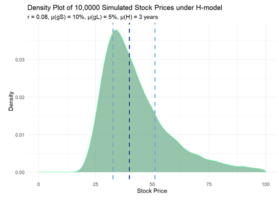
Here is an example. I am using a variation on the two-stage dividend discount model called the H-model. My code is here (TBA) on my blog. My initial static assumptions are the following: a $1.00 dividend starts by growing at 10% but that growth fades to 5% over six years (the half-life is three years) then exhibits stable growth at 5%, while the discount rate is 8%; i.e., gS = 10%, gL = 5% and H = 3 years. However, in the simulation these are means with modest standard deviations (see code). Over 10,000 simulations, assigning modest variability to three variables results in distribution with interesting properties:
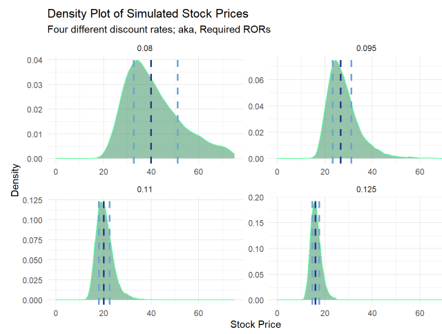
Next I used assumed four different discount rates: {0.08, 0.95, 0.11 and 0.125}. We can see the effects in this faceted plot. Interestingly, a high discount rate (r = 0.125) compresses the distribution toward lower values (of course) but with less dispersion.
Conclusion
We started with the basic self-refencing relationship between present value and a vector of future values, where they are linked by a single discount rate. My tour of (mostly) theoretical approaches aimed to show that future values, from a risk measurement perspective, are more interesting due to (i) their uncertainty and (ii) our subjectivity. Risk-neutral valuation is elegant but ultimately academic. We can increase the discount rate to compensate for risk, but this more suited to valuation than risk measurement (per the distinctions table at the top). Trees can explicitly model a volatility assumption, and we can formally add a risk aversion coefficient, but both attach with drawbacks. Ultimately, simulations are probably our best approach if we want to incorporate (at least) some realism at the cost of model risk and complexity. Risk measurement isn’t easy. See you in the next chapter!
In one sense, the difference between future value (FV) estimations and present value (PV) calculations is a matter of emphasis. We may need FV estimates to generate PVs, after all. Still, there is a often a big practical difference in the process and output between prioritizing today’s estimate versus tomorrow’s range of possibilities. For example, in public company investing where liquidity is high, reliance on valuation multiples effectively relegates long-term risk factors into a discretionary overlay or risk/reward synthesis. In accounting, for the sake of noble principles, fair value measurement can generate present values (e.g., employee stock options) that are economically dubious if not unusable.
Jorion, Philippe. Value at Risk, 3rd Edition. Here’s his table:
Knightian uncertainty (https://en.wikipedia.org/wiki/Knightian_uncertainty)
Normally we use present value (PV) and future value (FV) but I don’t want to suggest multiplication, as in P*V or F*V. For financial exam candidates who still somehow in 2024 need to suffer the use of a calculator (e.g., TI BA II+), the time value of money keys tend to occupy the same row: [N], [I/Y], [PV]. [PMT], [FV]. In a bond context, FV can also stand for face value.
I realize there is a common distinction between price (the bid/ask; what you can pay) and value (an asset’s fundamental or intrinsic worth), but I prefer to refer to the difference between model (aka, theoretical) price and its market price.
Probably the correct way to write this (I’ve written thousands of bond questions!) is something like “assumes a zero-coupon bond with a face value of $100. If the bond’s time to maturity [aka, remaining maturity] is five years and the yield is 5.0% per annum with continuous compounding…”. But the reader typically understands that term is years to maturity, and the reader definitely knows that 5.0% is annualized. But notice that we do need to specify the compound frequency: if we write “5.0% yield” then we can expect everybody to assume per annum, but this definitely does not connote an annual compound frequency. To write “5.0% yield” is to provide an incomplete specification!
And these are close enough. The first derivative is linear so the difference is the convexity that we aren’t capturing.
The inspiration for this two-step risk-neutral binomial model is John Hull's chapter on binomial option pricing (OFOD, Chapter 13, 11th Edition), although his concepts are not unique to him; e.g., Kolb
In other words, a US Treasury bill. It’s popular to use US Treasuries for the risk-free rate, but it’s not the tendency of expert practitioners due to the regulatory factors and favorable tax treatment that distort Treasury rates. For example, derivatives traders use overnight rates.
Lambda, λ, is default intensity; aka, hazard rate. It is an instantaneous conditional default probability. The credit risk approximation given by λ ≈ z/LGD in discrete (normal) time becomes an equality in continuous time when LGD = 100% where we can show that λ = z. As such, in continuous time with no recovery, the 3% spread is equal to an instantaneous conditional default probability of 3%.
At the risk of theoretical simplification, TBA
Risk/return: Note about factor theory [Ang] and the low volatility anomaly; i.e., when less risk associates with higher reward, we should pay attention
ex ante versus ex post, Sharpe ratio. Also, the utility function is subjective but
ChatGPT 4o gives this good itemization of the drawbacks to this highly theoretical approach