
Nearest neighbors (k-NN) for classification
This algo is a lazy learner (it doesn't actually train to build a model) but it's intuitive and handles many features.

Contents
To predict loan repay/default as function of income and credit score: it’s easy to visualize the hyperparameter choice (k = ?) in this two-feature space.
To predict cancer diagnosis with 30 features: Euclidean distance generalizes to many dimensions where the math is still easy but visualization isn’t.
To illustrate k-NN, I created synthetic borrower data (here’s the code for this post). My dataset includes 100 borrowers with two features, credit_scores and incomes. The target variable is a binary, label, that indicates whether the outcome was repay or default.

My code shows that I also added a bit of random noise (10%) to a rule that otherwise assigns repay to the high credit/income borrowers. These 100 borrowers are the training set displayed as green/red points in the scatterplots below. Subsequently, I invented a single new borrower with an income of (Y=) $41,000 and a credit score of (X=) 605. We want to predict whether (s)he will repay or default. This is supervised learning because the training set (n = 100) is already labeled (= repay | default) and we want to make predictions on our testing set, which happens here to include only one borrower. This test borrower is the blue triangle in the scatterplots below.
You’ll notice that all of my points—including the test borrower—are standardized: when we measure distance, we don’t want the income feature to dominate merely because its scale is larger. In this case, our test borrower is given by {X = 605, Y = 41000} → standardized {X(Z) = -0.912, Y(Z) = -0.857}. Unless we have a specific reason, we should scale1 features in the k-NN algorithm.

If the test borrower were located in the upper-right quadrant of the scatterplot (high income, high credit score) or further in the lower-left quadrant (low income, low score), we’d find it super easy to predict whether (s)he repays. But this test borrower is somewhere nearer to the middle. How shall we predict?

The k-nearest neighbors (k-NN) offers a simple plan: identify the k-nearest neighbors and let them vote. If most of those neighbors repaid (defaulted), the k-NN predicts the test observation will repay (default).
An unsophisticated thumb rule suggests we might set k = sqrt(N), so let’s do that and poll the k = sqrt(100) = 10 nearest neighbors. As plotted below, among these ten neighbors four repaid but six defaulted. Consequently, given this training set, 10-NN predicts default for this test borrower. We barely avoided a tie, and learned why we might prefer an odd number of neighbors when the target class is binary; e.g., default or repay!

Before I show you smaller and larger neighborhoods, 5-NN and 15-NN, let’s examine the 15 nearest neighbors as a dataframe. See below. This is just the original training set except it is sorted by an additional final column, distance, that I added to the dataframe. The first column is the original row identifier (row id) that’s out of sequence due to the sort by distance. The second through sixth columns are the training data: two raw features (credit_score, income); those same features standardized (credit_score_std, income_std), and the label (repay | default).

Among the 100 training observations, the nearest neighbor (to the test borrower) is the eighth (in the original) observation located at {credit_score = 611, income = $41,988} → Z = {-0.804, -0.759}. The final column, distance, is the Euclidean distance between the test borrower and this (training set’s) observation. This literally nearest neighbor has a distance of 0.145 as given by SQRT((-0.804 - (-0.912))^2 + (-0.759 -(-0.857))^2).
Each new test point has a different vector of distances to the training set. Our single test borrower, located at raw point {X = 605, Y = 41000}, is represented in my code by {x_std = -0.912, y_std = -0.857}. The distances_std is a vector of 100 Euclidean distances from this test borrower to each of the 100 training observations. By sorting—per the order() function—on that vector, I’m able to subset and create the k_nn dataframe.
distances_std <- sqrt((train$credit_score_std - x_std)^2
                          + (train$income_std - y_std)^2)

k15 <- 15
k_nearest_indices_std_15 <- order(distances_std)[1:k15]
k_nn <- train[k_nearest_indices_std_15, ]
As the k_nn (k=15) dataframe reveals, the prediction (aka, majority vote outcome) varies depending on how many neighbors vote. For this test borrower, the plots below show how k=5 neighbors predict repayment, but k=10 neighbors predict default, and k=15 neighbors revert back to predicting repayment!

A few notes:
In the k-NN algo, the choice of the hyperparameter k is the key choice. An intuitive approach here is the elbow method, while a more sophisticated approach is cross-validation (which I’ve introduced here in the context of regression).
Nearest neighbors (k-NN) is called a lazy learner because it does not build an explicit model. For example, I recently introduced decision trees which is also a classification algorithm; but the tree algo builds a tree model (with nodes and branches) that exists separately from its training data. It trains on data to build a model. But the k-NN doesn’t really train: at the time of prediction, it computes (and) sorts the distance vector.
Neighbors versus clusters: personally, I sometimes confuse k-NN with k-means clustering. Unlike k-NN, clustering is unsupervised and not lazy: it conducts an actual training (on the training set) and generates a model (with cluster centroids).
Cancer prediction
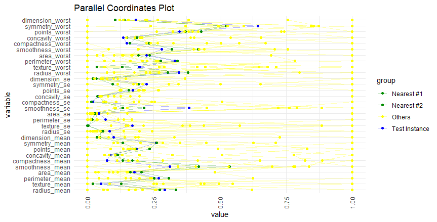
It was easy for me to visualize distance in two dimensions, but most datasets have many features. Euclidian distance generalizes to multidimensional space, but it becomes difficult (impossible?) to visualize. I briefly experimented with the visualization of multidimensional neighbors. The best I could find—on the quick—is the parallel coordinates plot below.
As my code shows, I used the dataset from my favorite machine learning introduction, Machine Learning with R by Brent Lantz, 4th Edition. This Wisconsin Breast Cancer Dataset has 569 observations and 30 numeric features that describe characteristics of the cell nuclei present in the image. The binary target variable is the diagnosis; i.e., benign or malignant.
The author did not attempt a visualization of this 30-feature dataset. He did parse the dataset into 469 training observation and 100 test observations. Also, his features are normalized (i.e., on a zero to one scale) rather than standardized like my borrower repay/default example.

Once the features are scaled, the code shows how easy it is to implement the k-NN algorithm. In fact, unlike my manual approach, we only need a single command. Per Brett Lantz, we can use the knn() function2 from the class package:
wbcd_test_pred <- knn(train = wbcd_train, test = wbcd_test,
                      cl = wbcd_train_labels, k = 21)
The sqrt(469) = 21.7 and he rounded to the odd number because the target class is binary; i.e., if he used 22, then a test vote could result in an 11-11 tie.
Below, I retrieved the first test instance and plotted its two nearest (Euclidean) neighbors in the training set. The test is blue and its two nearest neighbors are green. For comparison’s sake, I randomly sampled 10 other observations from the training set and colored them yellow. Although this obviously does not convey numerical distance, I think it’s a passable way to illustrate the proximity of the neighbors along these features.
I hope you enjoyed this introduction to k-nearest neighbor. See you next time!
To scale, we can normalize (aka, min-max scaling) or standardize (i.e., converting a value into its Z-score). The difference turns on outliers. Under normalization, you can train on a feature with bounds {0,1} but a test feature could fall outside these bounds. Under standardization (which I prefer as the default choice), outliers are treated as such rather than compressed.
We can see why this is lazy learning and “train” is a misnomer in k-NN. In my decision tree introduction (code here), the analogous function is “fit2 <- rpart(Dividend ~ ., data = my20firms, …)”. But that rpart() function trained to build a model that is stored in the list object called fit2. Subsequently the fit2 object (model) is used to make a prediction. But here the knn() goes directly to prediction by computing/sorting the observations in the “training set”.